PDF Types

SunSolve-P90 permits five types of PDFs: constant, Gaussian, skewed Gaussian, Weibull and arbitrary. Example distributions are shown in Figure 4.2.

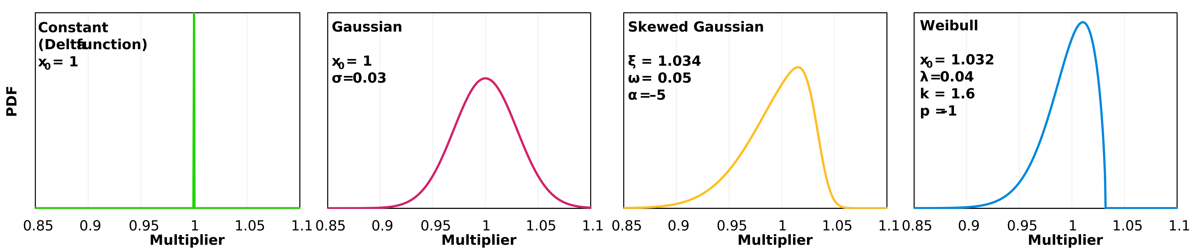
Figure 4.2: Four probability density functions. In these examples, each has an integral of 1 and a P50 of 1.

Constant

A multiplier of x = x₀ is assigned to all simulations.¹

Gaussian

The Gaussian function is defined by an offset x₀ and a standard deviation σ,

$$\text{PDF}(x)=\frac{1}{\sigma \sqrt{2\pi }}\exp (-\frac{(x-x_0{)}^2}{2{\sigma }^2})$$

The offset x₀ is also the mean of the distribution because a Gaussian is symmetric about x₀.

Skewed Gaussian

The skewed Gaussian function is defined by three variables, α, ξ, and ω.

$$\text{PDF}(x)=\frac{1}{\omega \sqrt{2\pi }}\exp (-\frac{(x-\xi {)}^2}{2{\omega }^2})[1+\alpha \cdot \frac{x-\xi }{\omega }]$$

The variables are sometimes referred to as the shape α, location ξ, and scale ω. When α = 0, this reverts to a Gaussian, where x₀ = ξ and σ = ω. When α > 0, the distribution is skewed such that the positive tail is ‘longer’ than the negative tail; and when α < 0, the negative tail is longer.

Weibull

A conventional Weibull function is defined by two variables, λ and k,

$$\text{PDF}(x)=\frac{k}{\lambda }{\left(\frac{x}{\lambda }\right)}^{k-1}\exp (-{\left(\frac{x}{\lambda }\right)}^k)$$

for x ≥ 0 and PDF(x) = 0 for x < 0.

In SunSolve-P90, however, we expand the Weibull function to include an offset x₀, and a polarity p so the tail of the function can be in either the positive or negative direction²

$$\text{PDF}(x)=\frac{k}{\lambda }{\left(\frac{p(x-x_0)}{\lambda }\right)}^{k-1}\exp (-{\left(\frac{p(x-x_0)}{\lambda }\right)}^k)$$

where p is either +1 or –1.

The value x₀ is therefore the point at which the distribution is zero (the discontinuity), and thus, when p is +1, PDF(x) is non-zero for x ≥ x₀ and zero for x < x₀; and when p is –1, PDF(x) is non-zero when x ≤ x₀ and zero for x > x₀.

Arbitrary

The user can also load their own uncertainty distribution, PDF(x), as a set of datapoints in the form {x, PDF}. The integral of the PDF(x) need not be unity.

Footnotes

1. If you’d prefer to treat this option as a function, then consider it to be a delta function centred at unity, PDF(x) = δ(x – x₀). ↩

2. The Weibull can be modified to have a similar form of the Gaussian distribution using x₀ = μ and λ = σ√2. ↩