Jupyter Notebook Walkthrough
This documentation provides comprehensive guidance for using SunSolve P90 via the “P90 Analysis” Jupyter notebook.
The notebook can be opened at this link in Google Colab. Google Colab provides a local, isolated virtual environment to access SunSolve P90, your inputs and results in this notebook will not be visible to anyone else.
A Jupyter Notebook Intro is also available for beginners to learn about Jupyter notebooks. A link is also provided to learn some useful keyboard shortcuts.
Note: the results from SunSolve P90 will not be ‘absolute yields’, instead giving relative yield values. You can supply your own absolute yield estimate to adjust plots to absolute (see ‘Converting to absolute yields’ section below).
Cell-by-cell workflow
Section titled “Cell-by-cell workflow”The analysis follows a structured workflow through numbered ‘code cells’. Each cell executes Python code to prepare and send your simulation request to SunSolve P90, then to analyse and plot the results.
- Login - Authentication
- Connection - Connect to SunSolve P90 and set up environment
- Load inputs - Define simulation parameters and system configuration
- Plot weather - Optional weather data visualization
- Visualize distributions - Optional distribution design tool
- Load uncertainty distributions - Define probability distributions
- Run analysis - Submit request and receive results
- Results - table of P-values - View requested P-values in a table form
- Results - histogram - Main result visualization
- Results - P-values vs Year - Multi-year trend analysis
- Export - Save results and backup notebook
- Further analysis - Custom analysis and additional visualizations
Step-by-step walkthrough in Google Colab
Section titled “Step-by-step walkthrough in Google Colab”-
Navigate to colab.research.google.com/github/pvlighthouse/SunSolveP90/blob/main/P90 Analysis.ipynb
-
Click the play button to run cell 1, installing the required libraries.
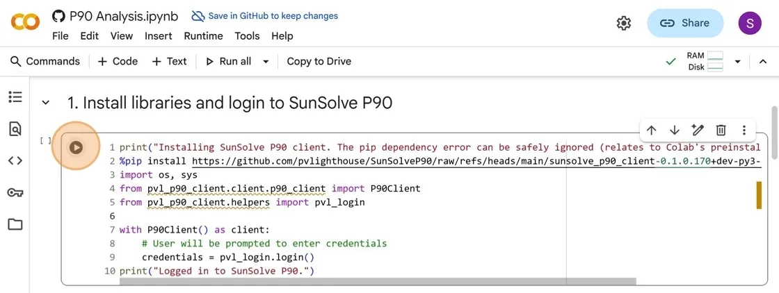
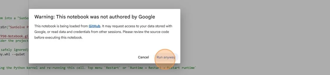
- A pop-up will warn that this notebook was not authored by Google, click “Run anyway” to continue.
Unfortunately, Google Colab has packages that have outdated dependencies, giving the below error. This can be safely ignored.
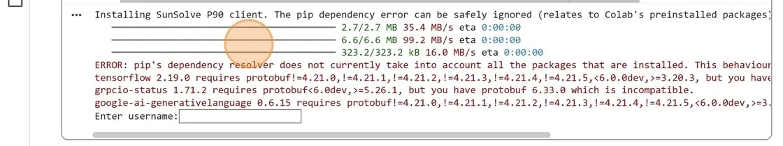
- Enter your PV Lighthouse email in the prompt and press
Enter. Then enter your password and pressEnteragain.

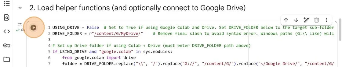
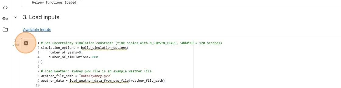
- Click the play button to run cell 2. This will load helper functions for analysing your results. Optionally you can configure Colab to connect to your Google Drive here, see “Google Drive integration” section below for details.
- In cell 3, add or adjust the available inputs to set up your yield model.
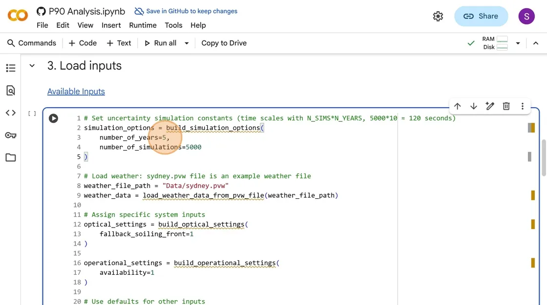
- Click the play button to run cell 3.
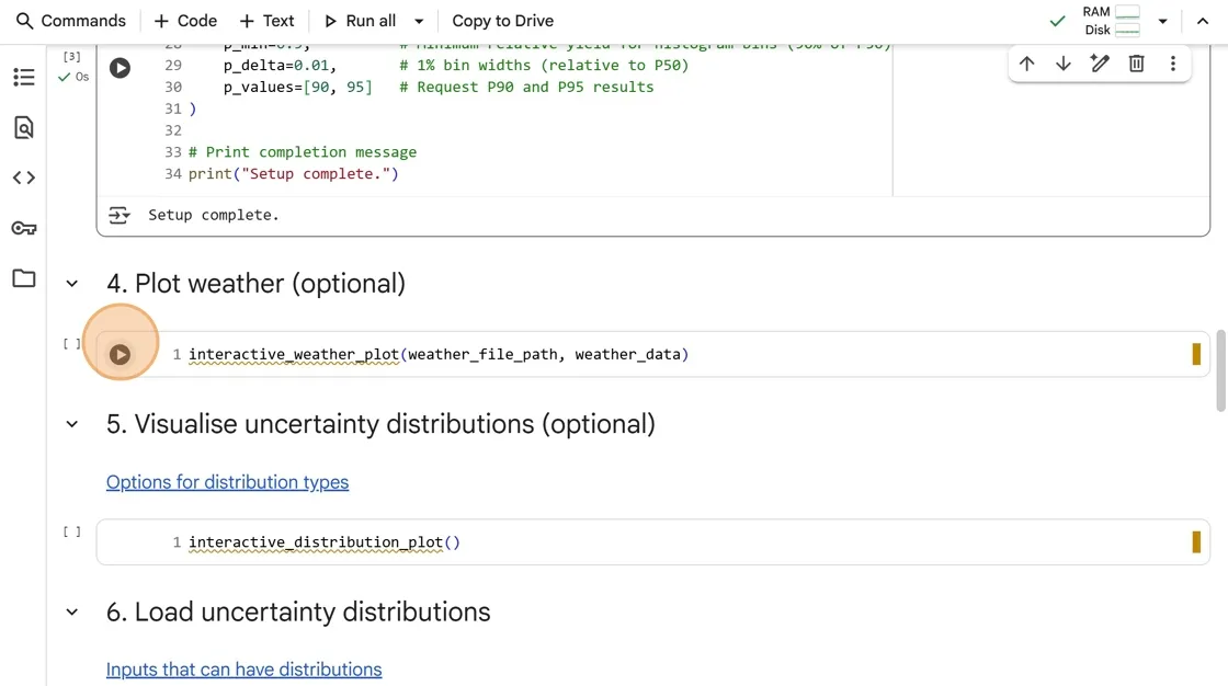
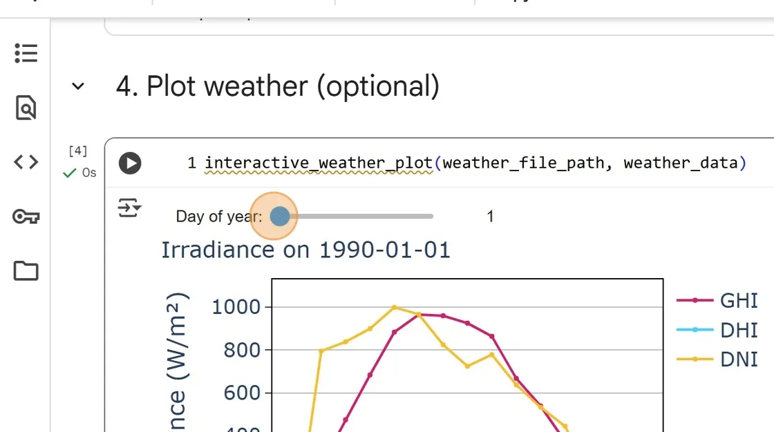
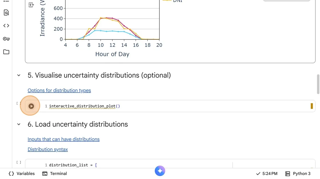
- (Optional) Click the play button on cell 4 to view daily plots of your weather file.
- Adjust the slider to select which day to plot.
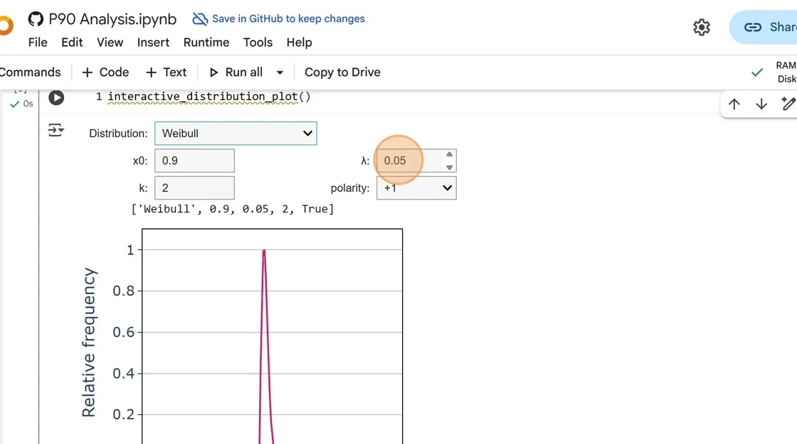
- (Optional) Click the play button on cell 5 to visualise uncertainty distributions.
- Select your desired distribution from the drop-down.
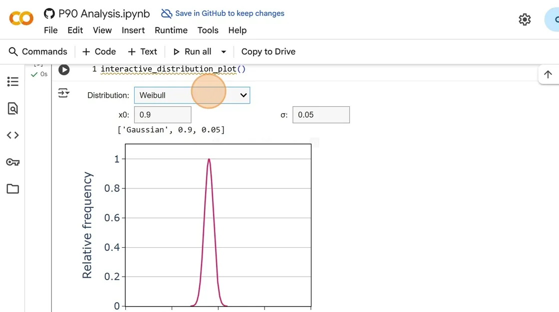
- Change any parameters you wish. The request syntax for the distribution is displayed in the plot title. You can copy this for cell 6.
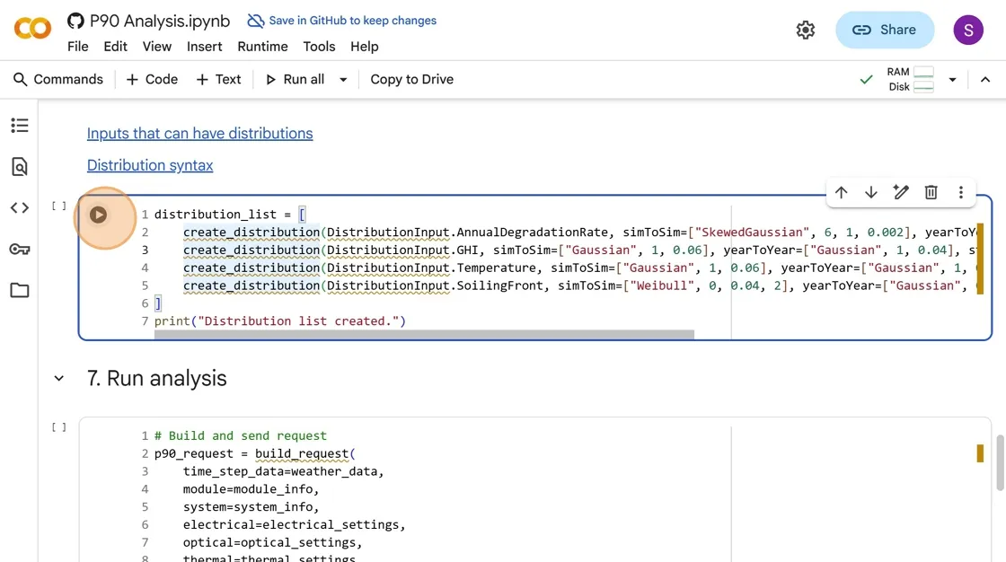
- Edit cell 6 to add uncertainty distributions to your desired inputs. See links for information about which inputs can have distributions and the syntax for specifying distributions. You can copy syntax from cell 5 and paste it here.
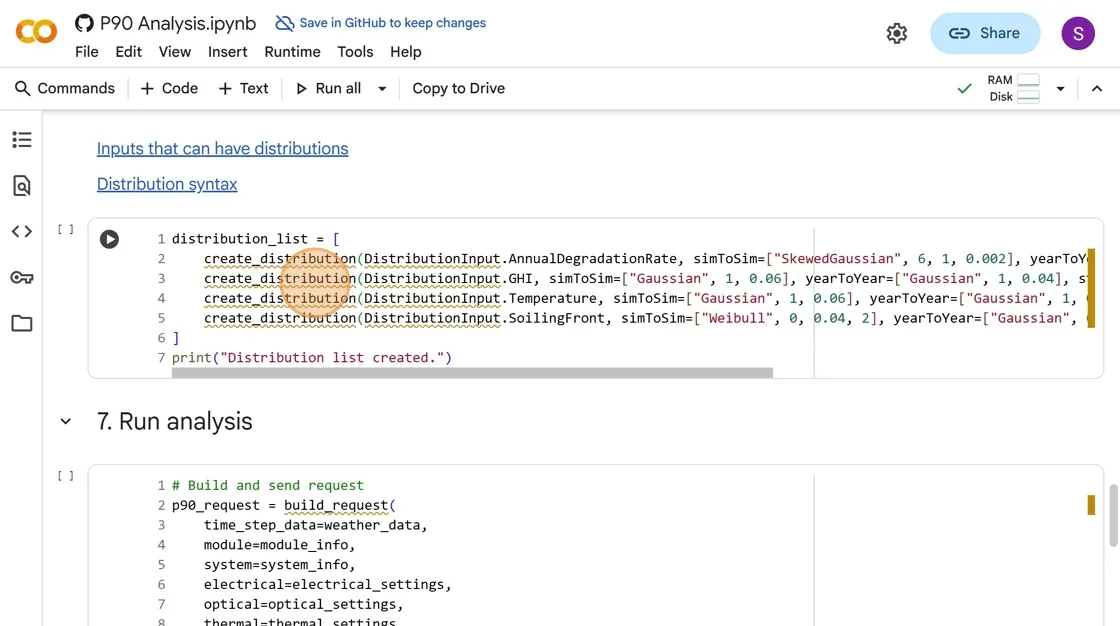
- Click the play button to run cell 6, saving your distributions as a list.
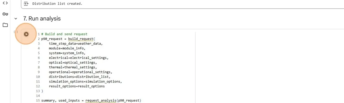
15. Click the play button on cell 7 to send your request to SunSolve P90 for simulation. It will return your result ‘summary’ and plot a table of requested P-values for all years.
16. (Optional) Change the year_one_yield value to your expected yield value (in MWh) if you have one, otherwise the plots will all be in terms of ‘relative yield’ (relative to year 1’s P50 yield). You can supply a yield_units= parameter to the plotting functions to change the units displayed.
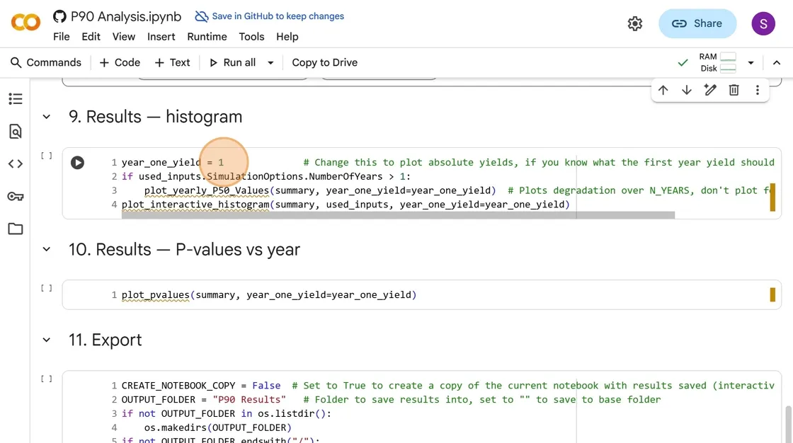
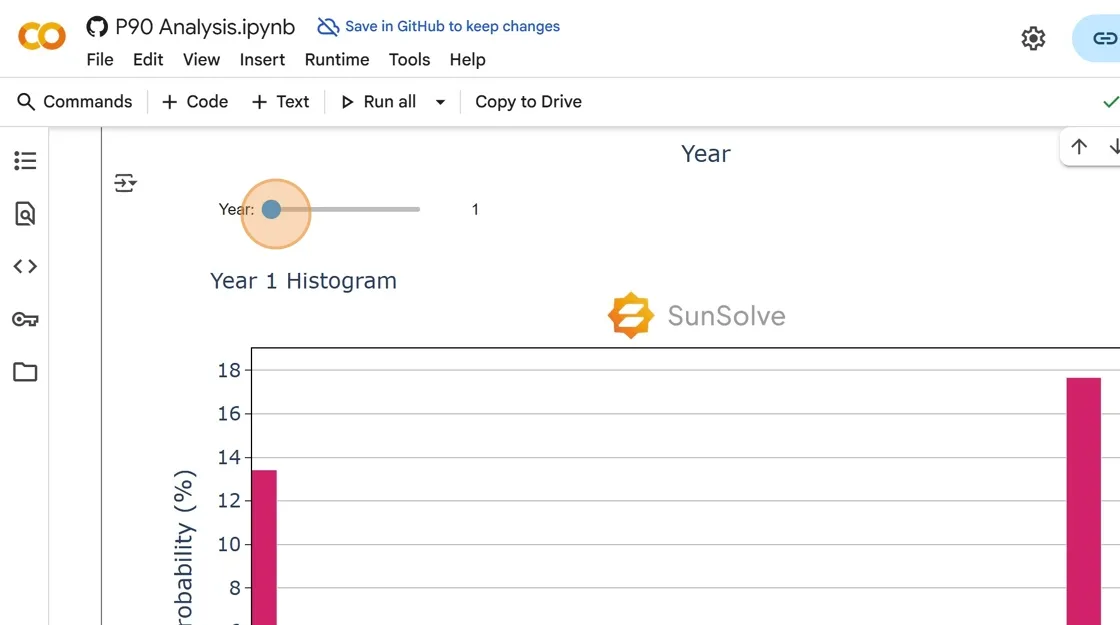
- Click the play button on cell 9 to plot the result histograms. It will also plot each year’s P50 (median) yield if you requested more than 1 year of simulation, showing degradation over time.
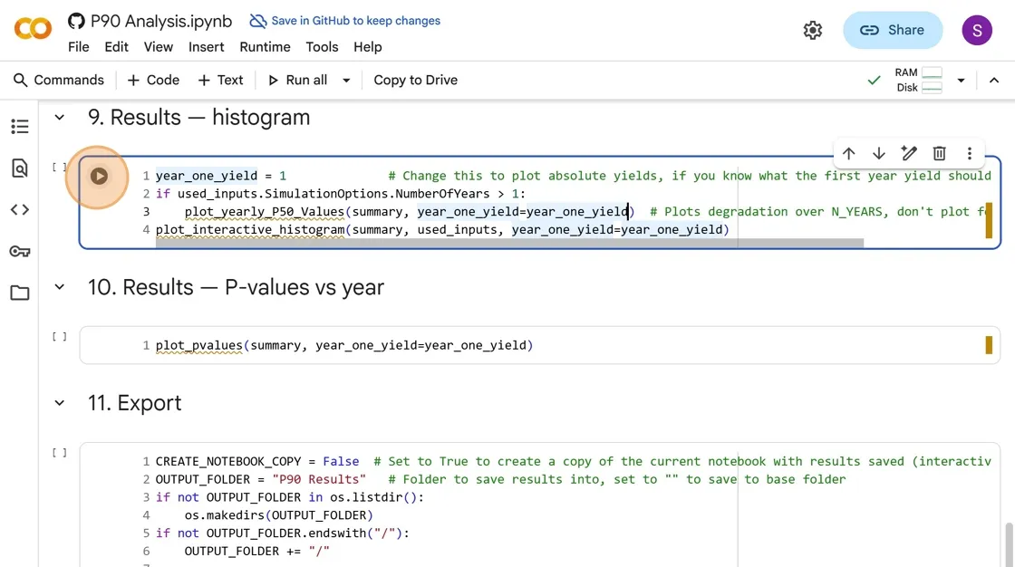
- Scroll through each year’s histogram using the slider. Each year’s histogram x-axis is relative to year 1’s P50 yield, but will show as absolute yields if you supplied a
year_one_yieldvalue.
- Click the play button on cell 10 to plot P-values vs. year, showing how different percentiles change over time due to degradation.
-
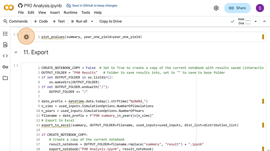
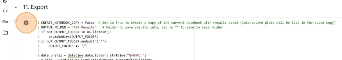
(Optional) In cell 11, you can change
CREATE_NOTEBOOK_COPYtoTrueif you would like to save a copy of your notebook. Make sure to save it before you click the play button. -
Click the play button on cell 11 to export your results to an Excel spreadsheet and (optionally) a copy of your notebook. Both will be saved to a “P90 Results” sub-folder by default.
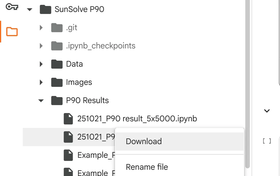
- To manually export your results from Colab, first click on the folder icon in the left pane.
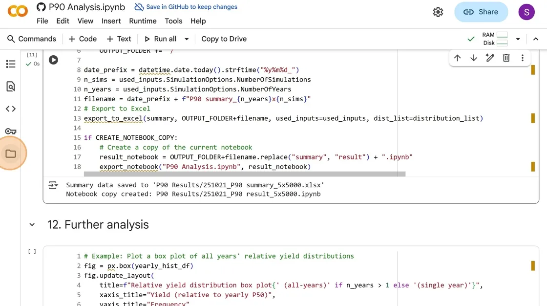
- Navigate to the “SunSolve P90/P90 Results” folder. If you can’t see it, try clicking the ↻ icon to refresh the folder view. You can then click the three dots to the right of a file to select “Download” and export the files to your local drive.
Google Drive integration
Section titled “Google Drive integration”For Google Colab + Drive users:
- Change
USING_DRIVEtoTrue - Change
DRIVE_FOLDERto the desired project folder on your drive- Paths starting with “G:” are attempted to be converted
- Make sure your path doesn’t end in a slash. Remove it if so (e.g. r”G:/My Drive/Notebooks/” -> r”G:/My Drive/Notebooks”), otherwise you will get a Syntax Error.
- You may need to manually adjust your mounted drive’s structure in Colab
- Run the cell, connect to your Google account, press
Continuetwice on the pop-up
Note: You can use Colab without Drive, but will need to manually download your results. Be careful of Colab’s 90-minute idle timeout for inactivity.
Converting to absolute yields
Section titled “Converting to absolute yields”Converting to absolute values:
- Change
year_one_yieldfrom 1 to your expected first-year yield in MWh - This scales all relative yields to absolute values
- You can add (for example)
yield_units="GWh"to a plotting function call to change the units if needed - Consider using SunSolve Yield for a physics-backed absolute yield estimate