Main solving algorithm

When a user runs SunSolve, they set simulation inputs across the Weather, Module, System, Field, and Options input pages:

1. Weather settings are documented in Weather options, which defines site location, weather, and atmospheric conditions.

2. Module settings are documented in Module cell layout, Module electrical layout, and Module frames and brackets, which define the geometry, optics, and circuit layout of the module.

3. System settings are documented in System types overview, System dimensions, and Ground albedo, which define layout, structural components, and optical boundary conditions.

4. Field-level electrical behaviour (module stringing and inverters) is described in System electronics; and

5. Algorithm options are documented in Yield simulation options and Weather options, including solar position and diffuse-light model settings.

After pressing “play”, these inputs are sent to a cloud-based server, which solves the yield and returns the outputs to the user’s computer.

The figure below depicts the high-level algorithm used by SunSolve to determine the energy yield. The figure shows the inputs in yellow, and how they feed into three major stages of computation:

Stage 1 solves the absorption of sunlight in every cell within the unit-system for a large range of solar positions.¹

Stage 2 solves the DC module output for every timestep within the date range. It combines the optical results of Stage 1 with the thermal and electrical models to produce IV curves for every module in the unit-system.

Stage 3 combines the results of the individual modules from Stage 2 to determine the DC output from strings of modules, and the AC output of the inverter.

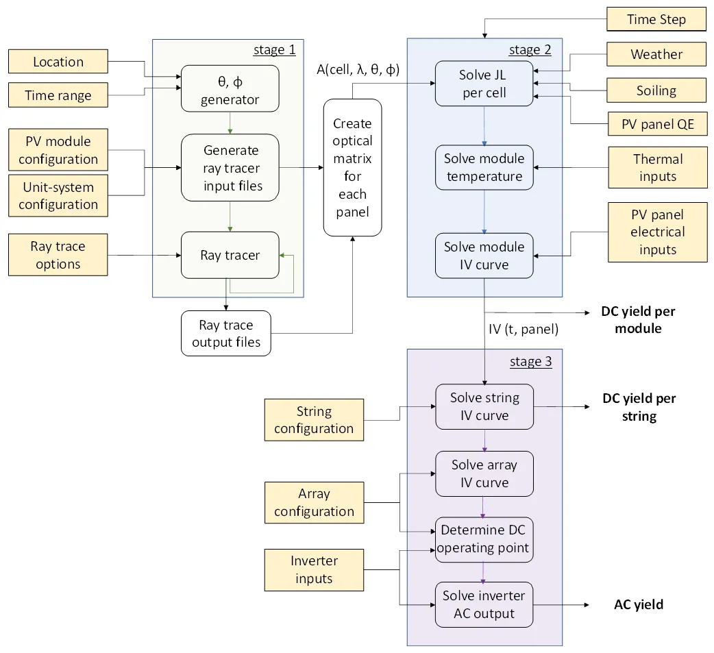High-level diagram of the stages of solving within SunSolve Yield

We now outline the details of each stage with links to the relevant technical-reference pages.

SunSolve calculates the energy yield as follows: It first loads weather from weather files (like TMY). It then calculates the solar spectra of direct and diffuse light, and the angle of incidence to the system. Next, it uses ray tracing and thin-film optics to determine the generation of current within each solar cell of the system. It feeds that light-generated current into an equivalent-circuit model of the system and determines the current–voltage output of each module. It also accounts for the thermal behaviour of the module by applying models to determine the module temperature from the environmental conditions and to adjust the electrical output accordingly.

Stage 1

Stage 1 solves the optics of the unit-system (System optics), which contains a group of modules whose optical and structural definitions are set in Module optics and Module electronics. The location and time range are used to determine a set of discrete sun positions along the solar arcs (Solar position). This is combined with the definition of the unit-system to create a set of static ray tracing models.² One such model is created for each point on the solar arc to determine the response to direct irradiance. Another model is created for the diffuse conditions which are always solved at this stage with isotropic irradiance³. The optics of each of these unit-systems is solved using the ray-tracing algorithm (Fundamental optics). This generates a set of ray tracing results which are combined into optical matrices which store the absorption in any cell within the unit system as a function of: (1) wavelength, (2) sun-position, (3) diffuse versus direct light.

Stage 2

Stage 2 solves the thermal and electrical result of every PV panel in the system at every timestep within the date range. The first step is to determine the light-generated component within each cell (Determination of cell light generated current). This involves application of the diffuse-light transposition model (Sky distribution of diffuse light), determination of the sun position (Solar position), interpolation of the closest three solar arc results, and combination of the incident spectra (Solar spectra) with module optical and wavelength-dependent current scaling definitions (Module optics). If soiling models (Soiling loss) are being used to de-rate the current, then they are applied at this stage to reduce the light-generated current of the cells. The operating temperature of each panel is then determined based on the balance of the heating and cooling mechanisms (Thermal model). The full current-voltage curve of every panel is then determined at the operating temperature by solving a SPICE circuit that contains an equivalent circuit for each cell (Equivalent circuit model) within a layout defined by the module circuit⁴ (Module electronics). Note that during this stage the DC maximum power output of each module is also determined at 25 °C and without the interconnection of cells within the module layout. The result of these two solutions is used to calculate the DC losses due to temperature and due to cell-to-cell mismatch. At the end of stage 2 the program has determined the IV curve at a single operating temperature for each module in the unit-system. The DC module yield is determined from these curves by assuming perfect maximum power point tracking and integrating over the specified time range.

Stage 3

Stage 3 solves the DC input and AC electrical output from a set of inverters defined within a complete field layout (System electronics). Each inverter input is connected to any number of parallel strings of series connected modules. In the first step the IV curve of each string⁵ is solved by combining the IV curves of the individual modules. In the second step the DC input to each inverter is solved by combining the string results in parallel and applying DC wiring losses. The AC output of each inverter is determined based on the DC input and the selected inverter model.

Footnotes

1. As evident in the figure, the approach is non-iterative. For example, the optical properties of the module materials are not modified once the module temperature is determined in Stage 2. ↩

2. For example, in an SAT the sun position is combined with the defined tracking algorithm to determine the module tilt. ↩

3. The number of diffuse models required is determined by the type of system. For fixed systems where the module tilt is independent of the sun position only one such model is needed. For tracking systems a solution is required for every sun position. ↩

4. This layout includes bypass diodes which can act to reduce the cell-to-cell mismatch losses that may be caused within the module due to spatially non-uniform irradiance. ↩

5. The string length may contain more modules than the definition of the unit-system. In this case the result of any panel may be included multiple times within the string. This is based on the definition of the string by the user. It may contain all the same panel or any mixture of the panels from within the unit-system. ↩