Using a plane-of-array sensor in SunSolve
A Plane-of-Array (POA) sensor is commonly used in PV system metrology to measure irradiance incident on a specific surface — typically the front or rear of a solar module. These sensors are usually pyranometers, capable of collecting light from all angles and across a wide spectral range (typically up to 4000 nm).
In SunSolve v7, there is no direct way to add a dedicated POA detector to the scene. However, a workaround is available using a specially defined module.
The procedure described here can also be used to extract the average front and rear irradiance across the entire module. This may be useful when comparing to other simulation tools like PVsyst or bifacial radiance.
A special module can be defined to act as a POA detector. This module is defined so that its light-generated current can be converted into irradiance. Simulations using this module focus solely on POA output and should not be used for full yield analysis. If yield data is needed, replace the POA module with the actual module model.
Spectral considerations
Section titled “Spectral considerations”SunSolve currently models light from 300 nm to 1200 nm, whereas POA sensors measure up to 4000 nm. This mismatch may introduce spectral errors, such as:
- A different ratio of irradiance below vs. above 1200 nm
- Wavelength-dependent effects in the scene (e.g., from albedo), especially for rear-facing POA sensors
These errors are minimised by calculating, at each timestep, the incident equivalent photon current density from 300–1200 nm (denoted as JL1200,GHI) and then scaling to estimate the total POA irradiance.
POA irradiance estimation
Section titled “POA irradiance estimation”The POA irradiance is thus estimated using:
Where:
- JL1200,POA — Light-generated current in the POA cell from 300–1200 nm
- JL1200,GHI — Equivalent photon current density of the incident irradiance (between 300–1200 nm) on a horizontal surface
- GHIAll — Total GHI across all wavelengths (e.g., up to 4000 nm)
Creating a module to act as a pyranometer in a specific location
Section titled “Creating a module to act as a pyranometer in a specific location”To behave like a pyranometer, the module should ideally:
- Collect light at a specific location
- Collect light equally from all angles (i.e., IAM = 1 at all angles)
- Provide a signal that can be calibrated to W/m² Additionally, in the unit system, it should:
- Reflect, transmit, or block light like a real module This is implemented in SunSolve using a complex module with a single cell that absorbs all incident light. The cell’s location is controlled via edge spacing to mimic a POA sensor. Surfaces away from the cell are defined to reflect light similarly to a typical module surface.
Example module definition
Section titled “Example module definition”The following section describes how to define a module that will approximate a rear-facing POA sensor located halfway down the module on the left hand side. It is set to collect light from all angles when they strike the cell area from the rear side. The upper front interface can be set to approximate module front-side reflectance. Alternatively it could be simply set to remove front side irradiance from the scene.
Steps to create
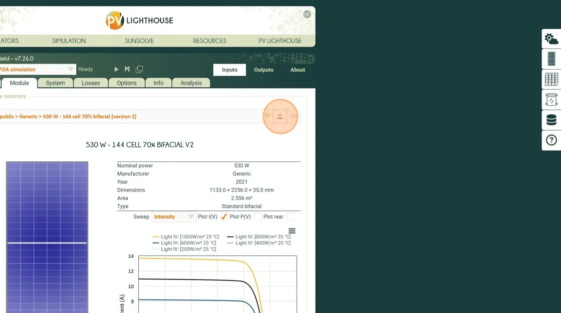
Section titled “Steps to create”1. Load a complex module into the user interface, for example ‘public > Generic > 535 W - 144 cell monofacial [version 2]’
2. Click this icon to send the module to the sidebar.
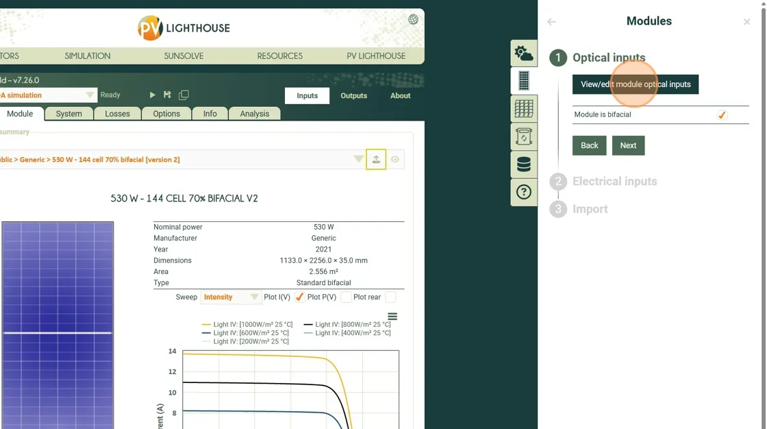
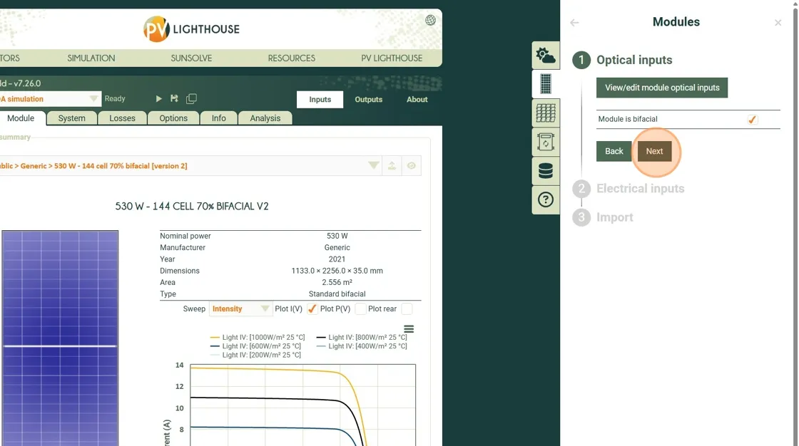
3. Click “View/edit module optical inputs”
4. Adjust the inputs to match the tables presented in the next section. Also shown in the images below.
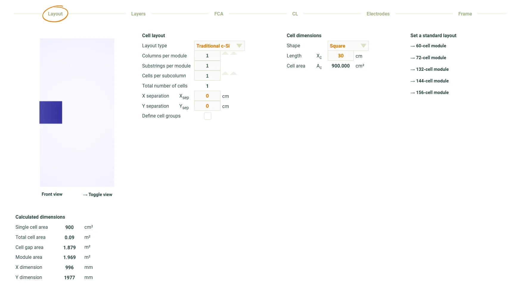
4.1. Set the layout to define a single sensor with a specific size.
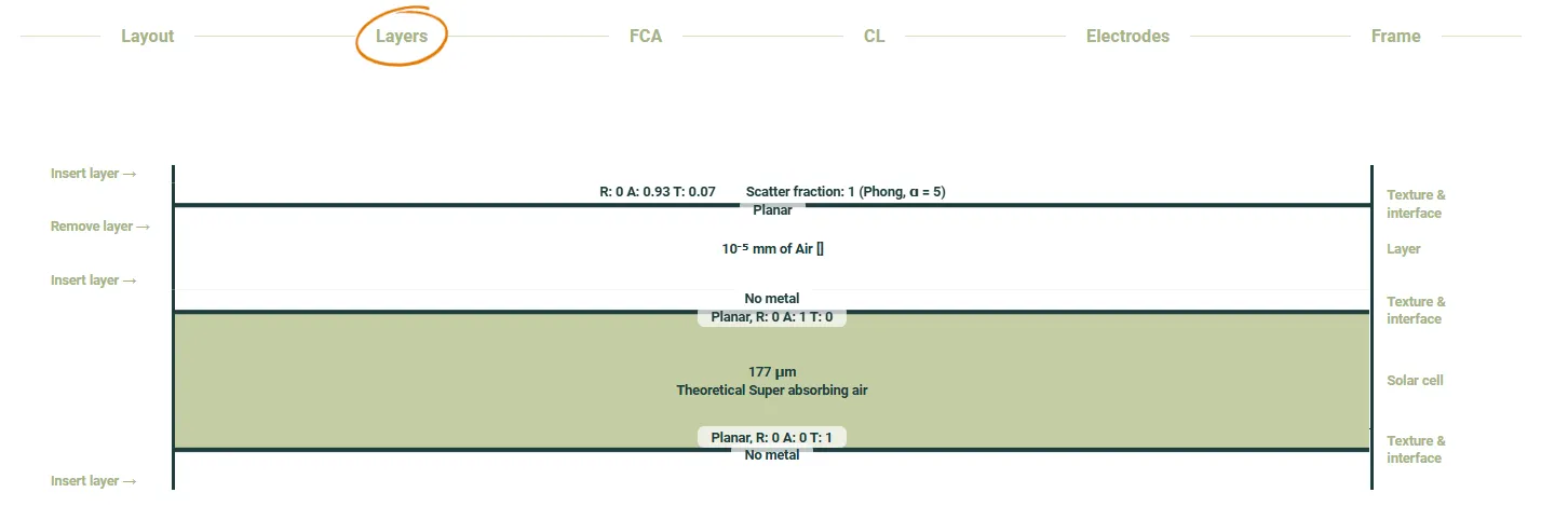
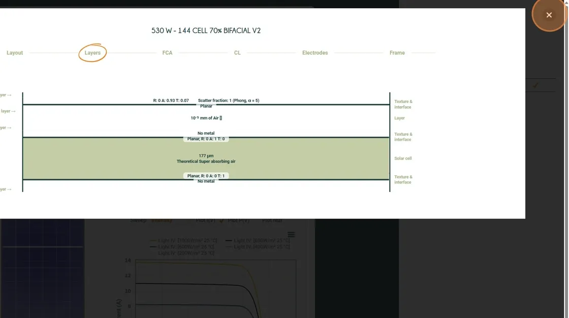
 4.2. Set the layers to define a super absorber and adjust the interfaces to either collect light or reflect it.
4.3. Set the collecting layer to have no wavelength dependence.
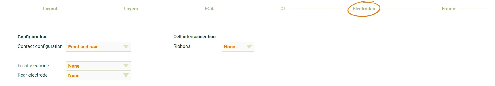
 4.4. Remove all electrodes.
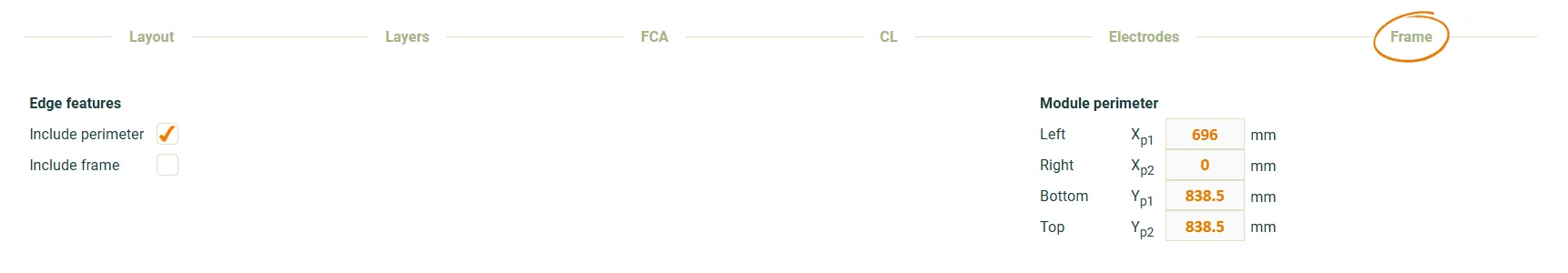
4.5. Remove any frame and set the perimeter spacing to position the sensor and define the final module size.
5. When finished adjusting the inputs, click this button to close the window.
 6. Click “Next”
 7. Click “View/edit module electrical inputs”
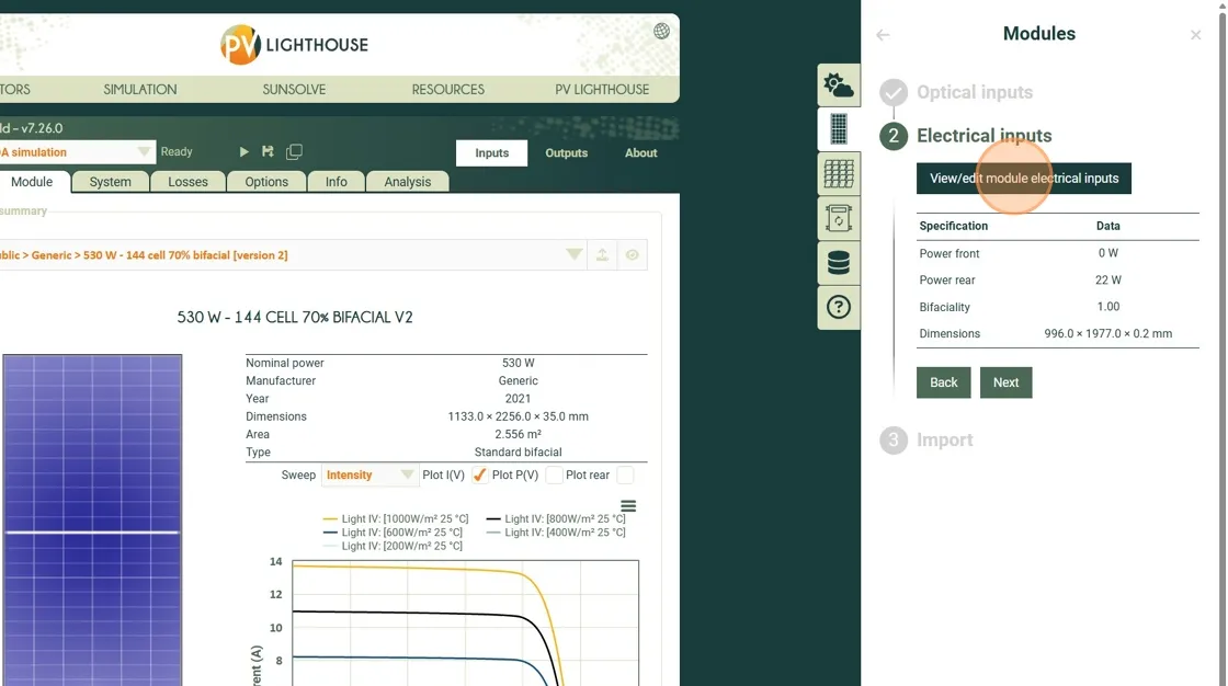 8. Adjust the inputs to match the tables presented in the next section. Also shown in the images below.
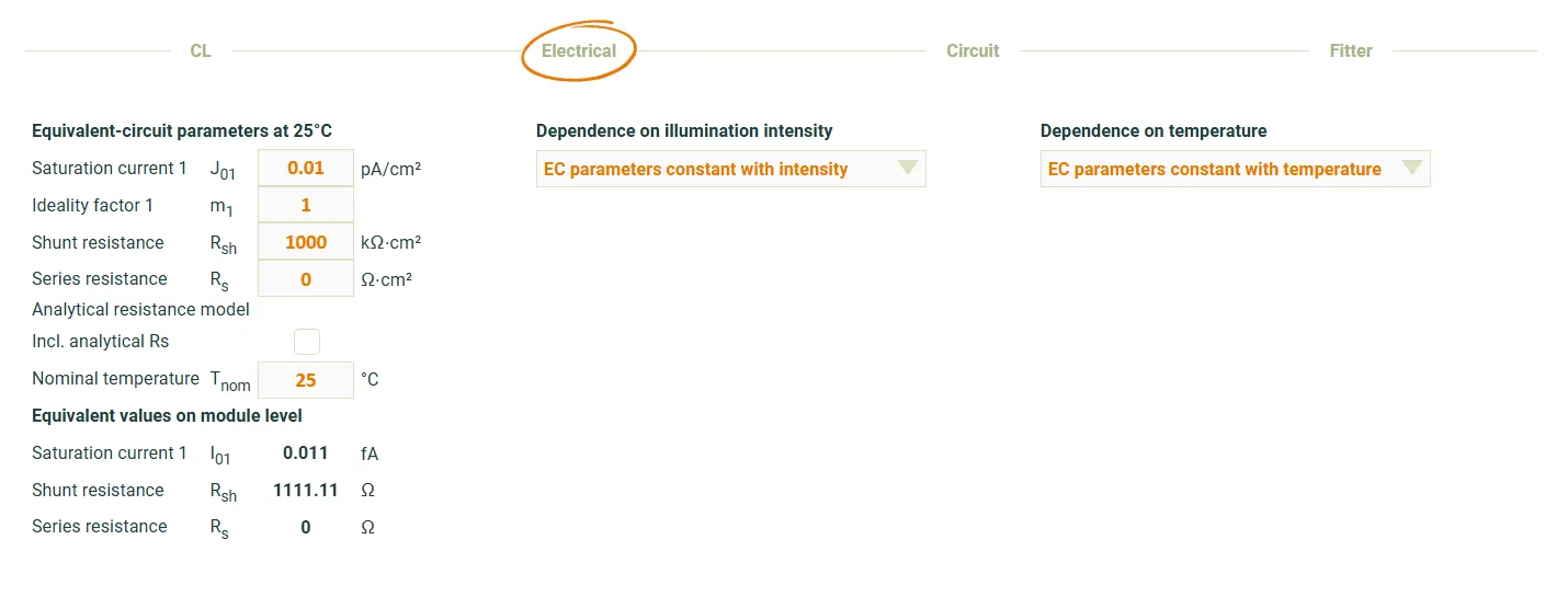
8.1. Set the electrical circuit to have no illumination or temperature dependence. Also set the circuit to give a linear response.
8. Adjust the inputs to match the tables presented in the next section. Also shown in the images below.
8.1. Set the electrical circuit to have no illumination or temperature dependence. Also set the circuit to give a linear response.
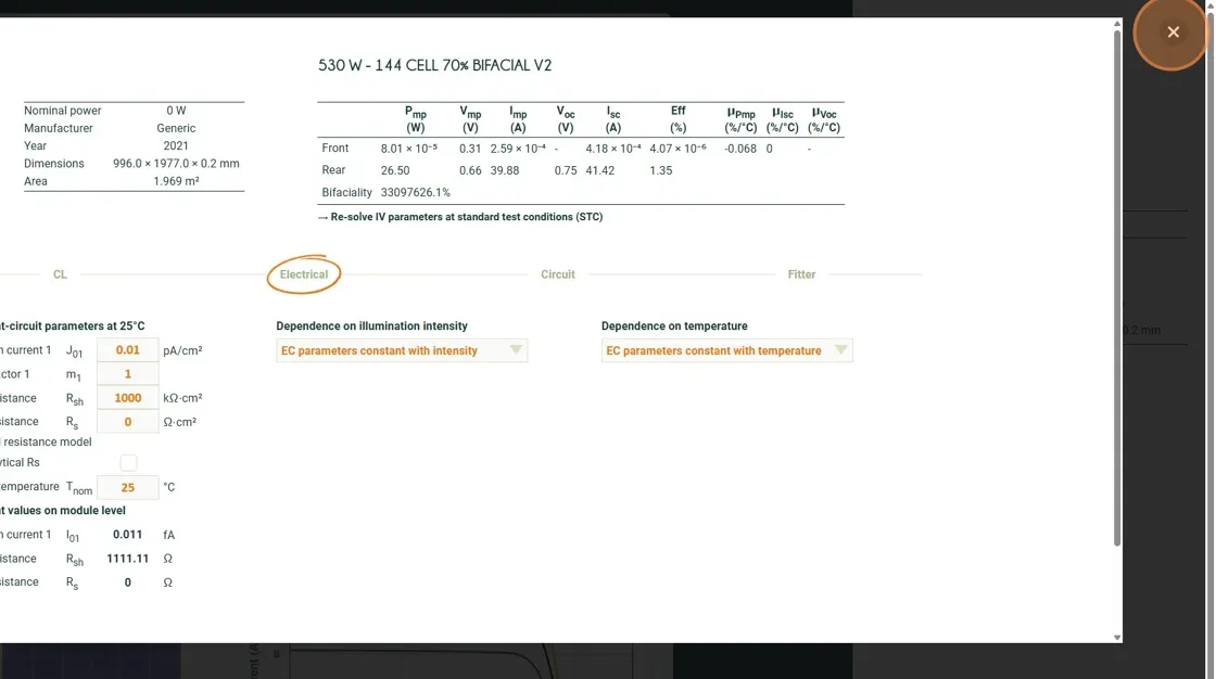
9. Click this button.
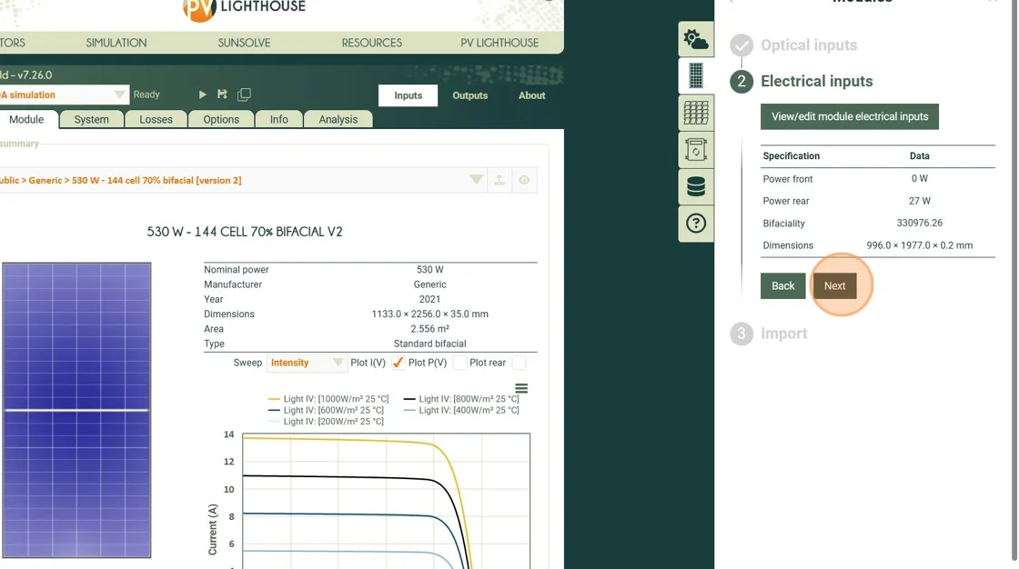
10. Click “Next”
11. Create a folder, give the module a name and when ready click ‘Import’
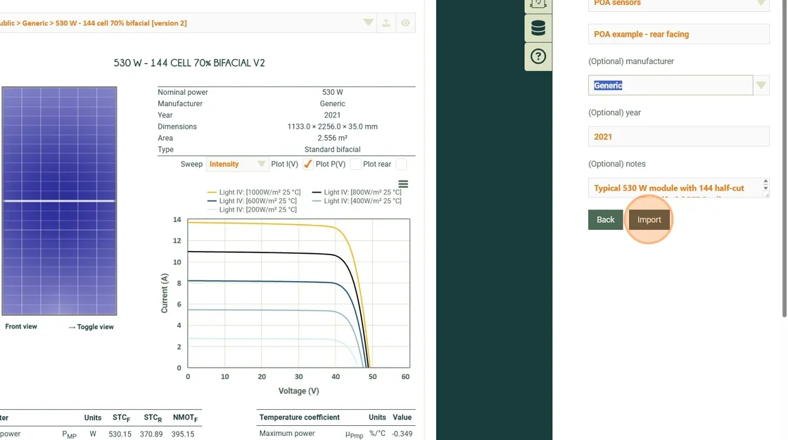
The special POA sensor module should now be added to your module library and ready to use.
Summary of optical inputs
Section titled “Summary of optical inputs”| Section | Parameter | Setting / Value | Notes |
|---|---|---|---|
| Layout | Layout type | Traditional c-Si | Not important for a single cell module |
| Columns per module | 1 | ||
| Substrings per module | 1 | ||
| Cells per subcolumn | 1 | ||
| Total number of cells | 1 | Single-cell detector | |
| X separation | 0 cm | Cell centered laterally | |
| Y separation | 0 cm | Cell centered vertically | |
| Define cell groups | ✗ | Not required | |
| Cell dimensions | Shape | Square | |
| Length | 30 cm | ||
| Cell area | 900 cm² | This is the area of the POA sensor | |
| Layers | Front structure | Air gap with upper interface | Set upper interface to approximate module surface reflection |
| Front interface | Planar, A = 1 (T = 0, R = 0) | Removes light from scene without contributing to JL | |
| Absorber layer | Theoretical Material “Super absorbin air”, 0.01 μm | Fully absorbing layer for POA response | |
| Rear interface | Planar, T = 1 (A = 0, R = 0) | Collect all light from all angles | |
| Electrodes | Contact configuration | Front and rear | |
| Front electrode | None | ||
| Rear electrode | None | ||
| Ribbons | None | ||
| Frame | Include perimeter | ✓ | |
| Include frame | ✗ | ||
| Module perimeter | Left (Xp1) | 696 mm | Defines cell position offset |
| Module perimeter | Right (Xp2) | 0 mm | |
| Module perimeter | Bottom (Yp1) | 838.5 mm | |
| Module perimeter | Top (Yp2) | 838.5 mm | |
| Resulting geometry | Single-cell “module” acting as a POA irradiance detector | Positioned via frame offsets to desired measurement location |
Summary of electrical inputs
Section titled “Summary of electrical inputs”| Parameter | Symbol | Value / Setting | Units / Notes |
|---|---|---|---|
| Equivalent-circuit parameters at 25°C | |||
| Saturation current 1 | J01 | 0.01 | pA/cm² |
| Ideality factor 1 | m1 | 1 | – |
| Shunt resistance | RSH | 1000 | kΩ⋅cm² |
| Series resistance | RS | 0 | Ω⋅cm² |
| Analytical resistance model | Disabled | (unchecked) | |
| Include analytical Rs | No | – | |
| Nominal temperature | Tnom | 25 | °C |
| Dependence on illumination intensity | EC parameters constant with intensity | – | |
| Dependence on temperature | EC parameters constant with temperature | – |
Notes on the input settings
Section titled “Notes on the input settings”Cell area
Section titled “Cell area”The cell area does not need to be exactly the same as the actual POA sensor. It should be good enough to be close to the correct size. The trade-off in this parameter is between acurately measuring in a specific location versus reducing the stochastic error.
Module area
Section titled “Module area”The total module area will be determined via a combination of the cell dimensions and the perimeter inputs.
Stochastic error
Section titled “Stochastic error”This approach may result in the SunSolve engine automatically choosing to run too few rays. This may result in unacceptable stochastic error. In this case please contact support@pvlighthouse.com.au to request permission to set the number of rays per solar arc manually.
Creating a module to record average irradiance
Section titled “Creating a module to record average irradiance”The average irradiance across an entire module area can be calculated for either simple or complex modules. However, for this purpose, it is recommended to load a simple module from a .pan file that matches the physical size of the module under test.
Incident Angle Modifier (IAM)
Section titled “Incident Angle Modifier (IAM)”If the irradiance calculation should exclude incident-angle effects, set the IAM to 1.0 for all angles. This can be done during the module loading process by editing the optical inputs as shown below:
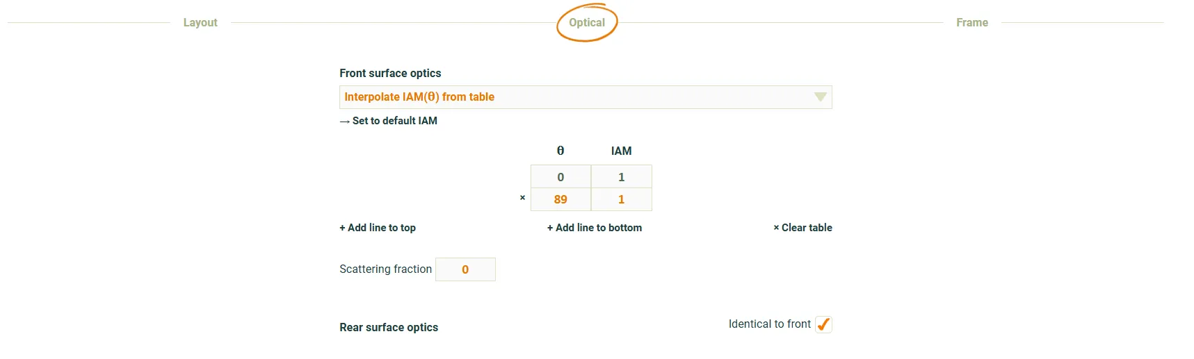
Note: Many simulation tools — including PVsyst and bifacial_radiance — do not apply IAM to the reported rear-side irradiance. In other cases, it may be included. Users should confirm how IAM is treated in their workflow. In real systems, rear-side IAM effects are always present, so applying unity IAM in SunSolve is purely for idealised or comparison studies.
Downloading POA Results
Section titled “Downloading POA Results”The equivalent POA irradiance can be exported in a CSV output file from the Time Series output tab.
Users should select the POA equivalent irradiance option in the Solve type dropdown menu.
Running this time series request will result in the equation above being solved for each time step.
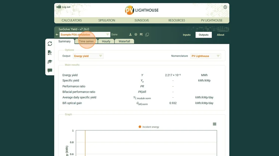
1. Run the POA simulation
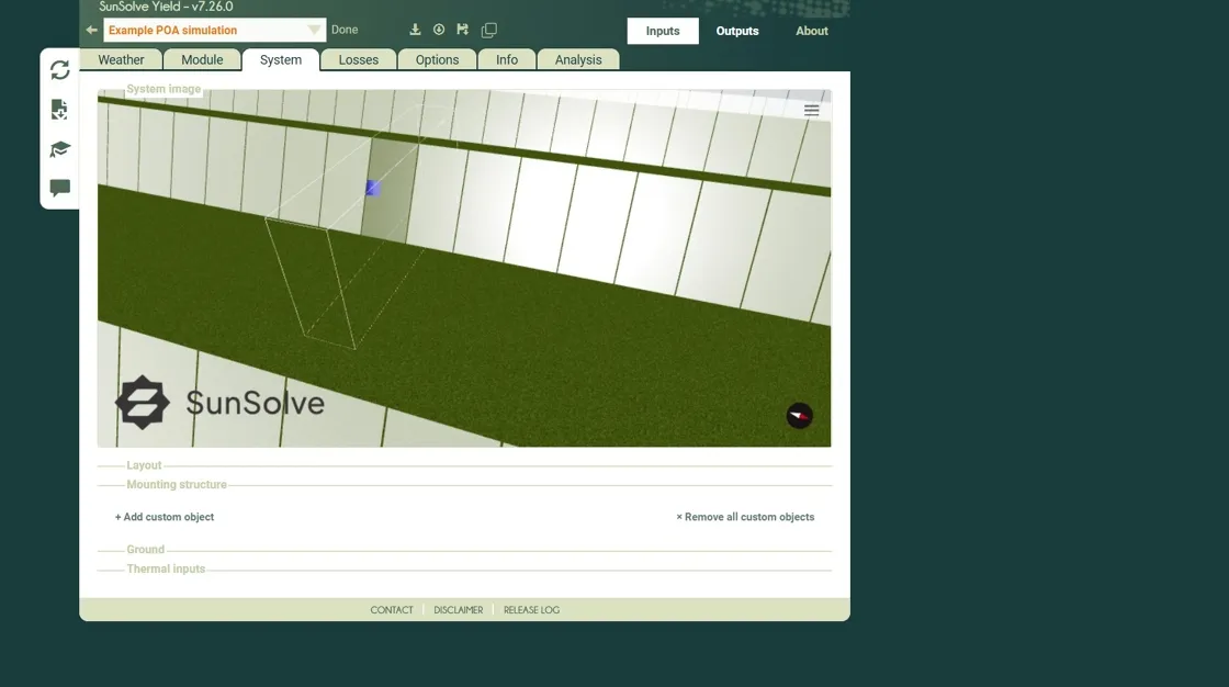 2. Click “Outputs”
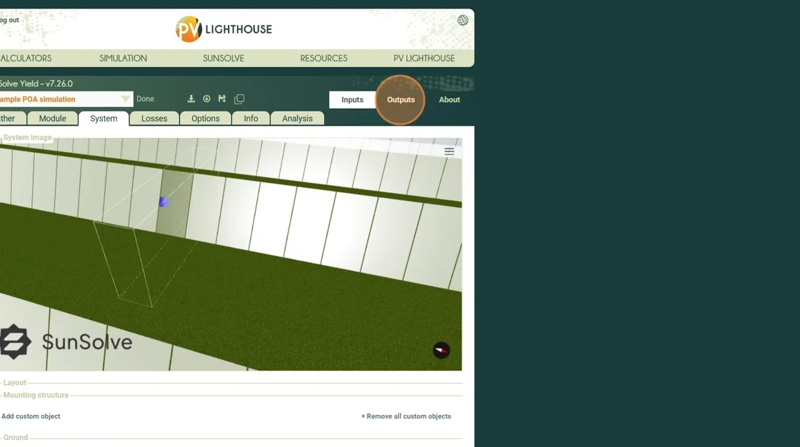 3. Click “Time series”
 4. Optionally click the “Select Date Range..” field to set a reduced date range. This can be useful if the POA download is too slow.
 5. Select the “POA equivalent irradiance” option for the “Solve type”
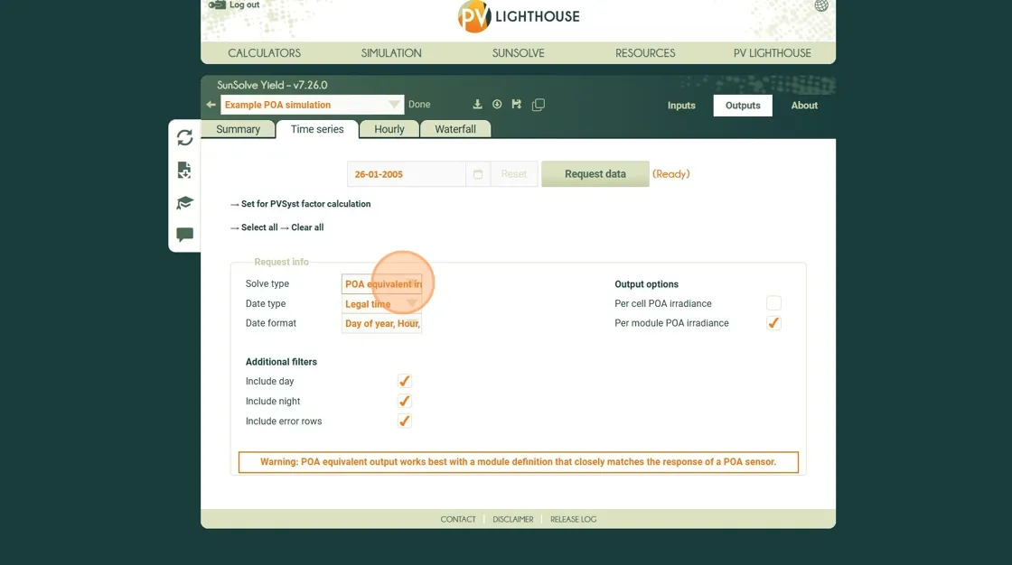 6. Click “Request data”
 This will result in the download of a csv file containing one row per time step per module in the simulation.
For each row there will be a value for the average front and rear irradiance on that specific module.
This will result in the download of a csv file containing one row per time step per module in the simulation.
For each row there will be a value for the average front and rear irradiance on that specific module.
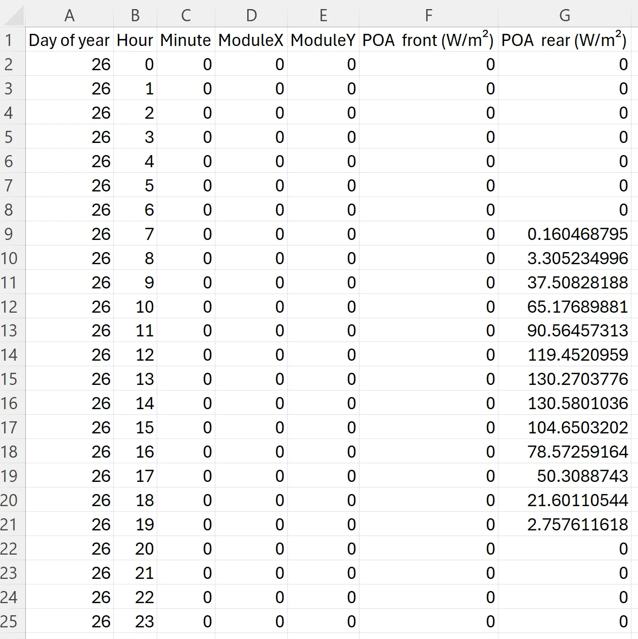 Example csv file contents after downloading POA equivalent irradiance for the localised POA module described above