Module current scaling in simple optical models

When using a simple module model in SunSolve, the optical behaviour of the module’s active region is solved with a normalised factor, usually an incident angle modifier. To ensure that this simplified optical treatment still produces realistic electrical results, a short-circuit current scaling factor (SF) is calculated for every simulation.

This page explains how that scaling factor is determined and how it connects the ray-traced absorption results to the expected electrical performance of the module.

Note that this calculation is not applied when using the complex module model.

Purpose of the scaling factor

The goal of the scaling factor is to match the optical absorption computed by the ray tracer to a known or target module current. Since simplified optical models cannot fully reproduce the complex internal structure of real modules, the scaling ensures that the resulting simulated short-circuit current (I_sc) remains consistent with laboratory or manufacturer data.

In short, it adjusts the optical absorption results to produce the correct level of current generation under standard test conditions (STC).

Overview of the calculation procedure

The scaling factor is determined using a sequence of physically motivated steps. Each step converts the optical absorption data into an equivalent module-level short-circuit current.

Step 1 – Normal-incidence ray tracing

A ray-trace simulation is first run on the module independent of the full system scene. Light is incident normally (θ = 0°) on the front of the module, and the absorbed fraction of photon current density at each wavelength in each cell is recorded.

If the module is bifacial, this process is repeated for illumination from the rear side.

Step 2 – Cell-level light-generated current

For each cell, the wavelength-dependent absorbed fraction A(λ, x) is combined with a quantum-efficiency spectrum QE(λ) to estimate the local light-generated current density:

J_{L,cell}(x) = \sum_{\lambda=300 \ nm}^{1200 \ nm} J_{photon}(\lambda) \times A(\lambda, x) \times QE(\lambda)

where

J_photon(λ) is the photon flux from the AM1.5g reference spectrum,
A(λ, x) is the fraction of absorbed light at wavelength λ in cell x, and
QE(λ) is the user-selected quantum-efficiency curve.

Step 3 – Unscaled module short-circuit current

The total unscaled short-circuit current for the module is obtained by summing the contributions from all N cells and accounting for the cell area and number of parallel strings P:

I_{sc,unscaled} = \frac{Single \ cell \ area}{N} \times P \times \sum_{x=1}^{N} J_{L,cell}(x)

Step 4 – Determine the scaling factor

Finally, the scaling factor is computed as the ratio of the unscaled simulated current to the target or expected short-circuit current (I_sc,target):

SF = \frac{I_{sc,unscaled}}{I_{sc,target}}

This wavelength-independent factor is then applied to all spectral calculations so that the simulated module reproduces the correct STC short-circuit current.

Quantum-efficiency options

The quantum-efficiency (QE) curve defines how effectively absorbed photons generate current. SunSolve provides several predefined QE profiles:

100% at all wavelengths — constant value, effectively no scaling is applied
Typical c-Si front — representative of high-efficiency PERC cells
Typical c-Si rear — representative of high-efficiency PERC cells measured from rear
FS Series 6 (CdTe graded) front — graded thin-film profile based on Series 6 module data

Each QE curve modifies the spectral weighting of absorption during current-generation calculations.

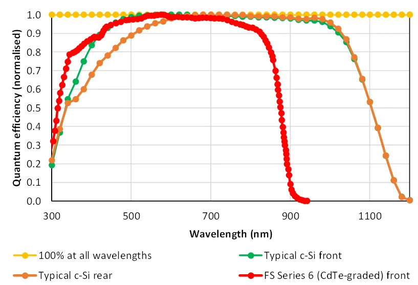Wavelength-dependent quantum-efficiency curves used for scaling in simple modules.

The crystalline silicon data is based on simulations within SunSolve of a typical PERC style high efficiency panel. The graded CdTe curve was extracted from the figure presented on the First Solar website for the Series 6 product.

Interpretation

The scaling factor (SF) acts as a bridge between optical and electrical domains.

A value of SF > 1 indicates that the simplified optical model under-predicts the target I_sc.
A value of SF < 1 suggests that it over-predicts.

Because the factor is derived from physical absorption data, it maintains consistency across both front- and rear-side illumination, enabling robust comparisons between bifacial and monofacial modules.