Key features

This page provides a detailed look at the main capabilities of SunSolve Yield. Each feature includes descriptions, context, and example diagrams.

---

Comprehensive System Modeling

SunSolve Yield supports multiple PV system configurations, each with distinct geometric and structural characteristics. The software accurately models fixed, single-axis tracker, and wave systems, capturing how these designs influence both optical and electrical performance. All simulations are performed in a fully 3D environment, which includes the rear-side (bifacial) collection of light.

By defining system geometry and layout in detail, users can explore the impact of module spacing, tilt angle, mounting height, structural shading, and inter-row shadowing on energy yield. Each configuration type includes its own structural components and modeling assumptions, described below. Users may also upload custom 3D objects derived from CAD files to represent unique or specialized system elements.

In all cases, SunSolve Yield uses forward ray tracing to accurately model the optical behavior of the scene. Light absorption is recorded on both the front and rear sides of every cell within each module, enabling detailed analysis of complex shading patterns and precise calculation of electrical mismatch effects.

---

Fixed Systems

Fixed systems have modules mounted at a constant tilt and azimuth. The structure typically comprises posts, rafters, and purlins that hold modules in a stationary position. This configuration is simple and widely used for ground-mounted and rooftop systems.

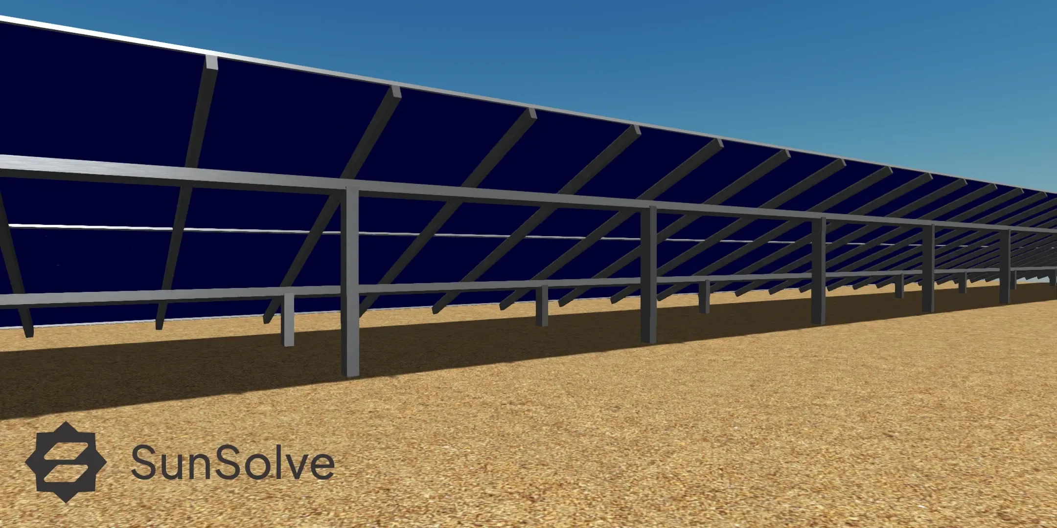
Figure 1 – SunSolve screenshot of a fixed-tilt PV system showing rear-side mounting structure including posts, rafters, and purlins.

---

Single-Axis Tracker Systems

Single-axis trackers allow modules to rotate about a defined axis, enabling them to follow the sun’s apparent motion throughout the day. The structure generally includes posts, torque tubes, and rails. Tracker systems improve energy yield by maintaining near-optimal module orientation.

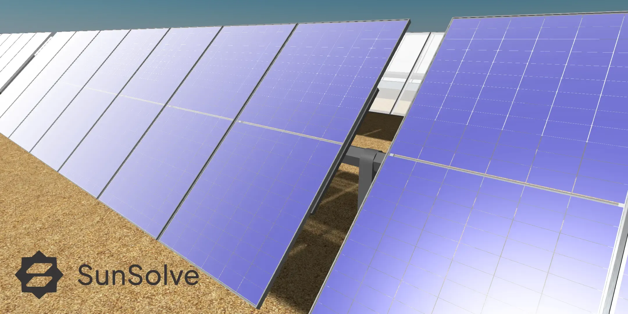Figure 2 – SunSolve screenshot of a single-axis tracker system viewed from the front.

---

Wave / Dome Systems

Wave or dome systems consist of paired module rows that face each other, forming a wave-like pattern. This configuration provides very high ground coverage. The structure commonly includes ballast blocks, rails, and joints. Despite being low to the ground, these system still provide some bifacial gain.

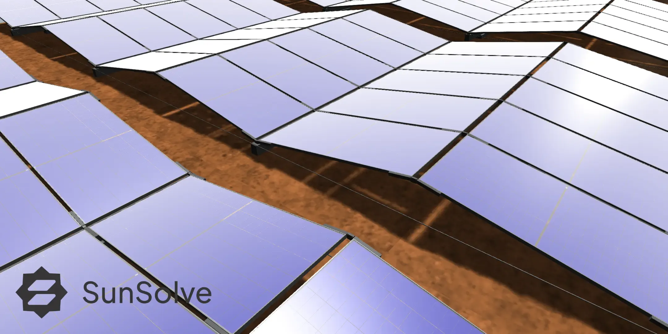
Figure 3 – SunSolve screenshot of an example wave configuration built to replicate the specialised 5B Maverick product.

---

Vertical PV

Vertical PV systems consist of modules mounted with a vertical tilt, typically facing east and west. This configuration is often used in agri-PV, fence-mounted, or building-integrated installations, where ground use, shading, or aesthetic constraints limit traditional layouts.

Vertical systems offer unique performance characteristics — they capture morning and afternoon sunlight more effectively, reduce self-shading, and can enhance bifacial gains through rear-side illumination. In SunSolve Yield, vertical systems can be modeled using the same geometric and optical framework as other configurations, allowing detailed analysis of orientation, height, spacing, and ground albedo effects.

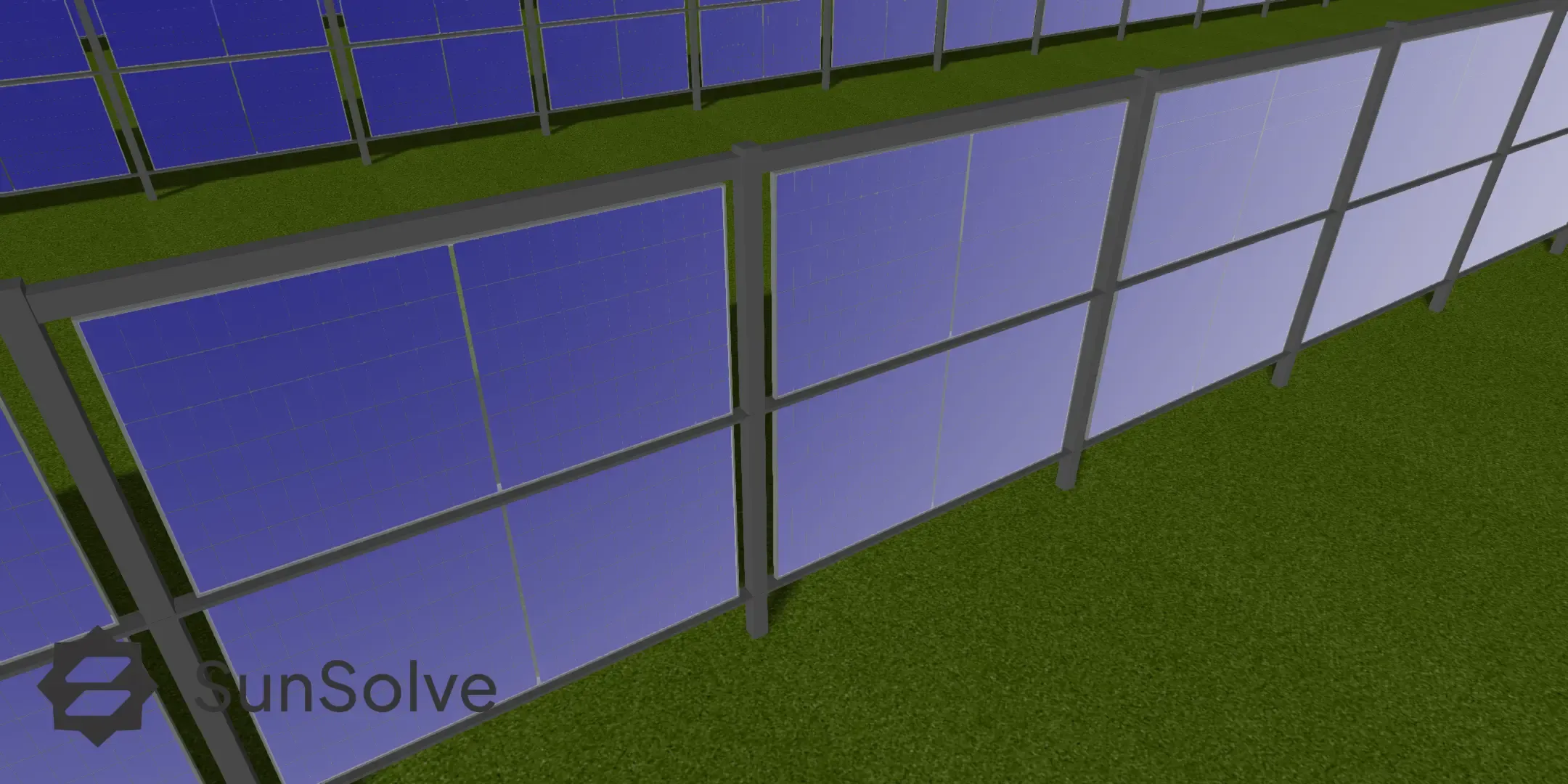Figure 4 – Example of a vertical east-west PV configuration modeled in SunSolve Yield.

---

Custom Structure

Structural objects can be uploaded from CAD designs, allowing a very high level of detail to be included in optical simulations. These may represent individual structural components or complete racking assemblies. Objects can be attached to the fixed or tracking elements of the scene, or alternatively to each module directly.

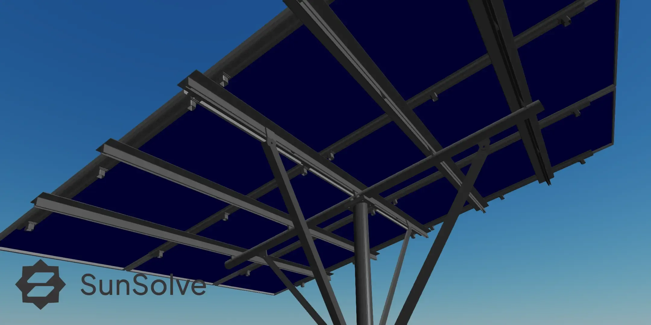
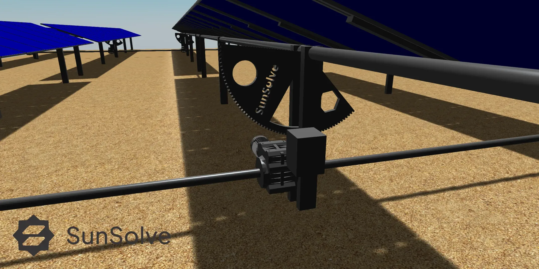
Figure 5 – Custom structures imported from CAD and integrated into the SunSolve scene.

---

Detailed Performance Analysis

SunSolve Yield provides a complete suite of analysis tools that quantify how effectively a photovoltaic system converts sunlight into usable electrical energy. Beyond overall yield and efficiency metrics, the software offers detailed visual and numerical diagnostics to trace the full energy path—from irradiance capture and module behavior to array-level losses and inverter output.

Together, the performance summary, waterfall energy breakdown, time-series outputs, and hourly heat maps give users a deep understanding of both short-term dynamics and long-term energy trends. These tools make it possible to pinpoint where optical, thermal, or electrical losses occur and to validate design choices with a level of physical accuracy unmatched by conventional yield models.

---

System Performance Summary

SunSolve Yield provides detailed performance metrics that quantify how effectively a PV system converts available irradiance into usable electrical energy.

The summary reports energy yield, specific yield, and performance ratio, along with bifacial indicators such as rear-side optical gain and bifacial performance ratio. It also breaks down irradiance inputs, DC/AC energy conversion, and system efficiencies, giving users a clear view of total yield, losses, and operational performance under realistic conditions.

---

Waterfall Energy Breakdown

The Waterfall chart provides a visual summary of the full energy flow through a PV system — from incident irradiance to AC energy output at the inverter. The upper section compares irradiance components, showing how the in-plane and rear-side irradiance relate to the global horizontal irradiance (GHI), while the lower section quantifies successive energy conversions and losses.

Each stage in the lower chart represents a transformation or correction: starting from the array’s nominal energy at STC, successive reductions are applied for optical, temperature, mismatch, wiring, and inverter losses, leading to the final available AC energy at the system output. Positive and negative bars highlight gains (such as bifacial contribution) and losses (such as inverter voltage limits or thermal effects), offering a clear diagnostic view of system efficiency and performance bottlenecks.

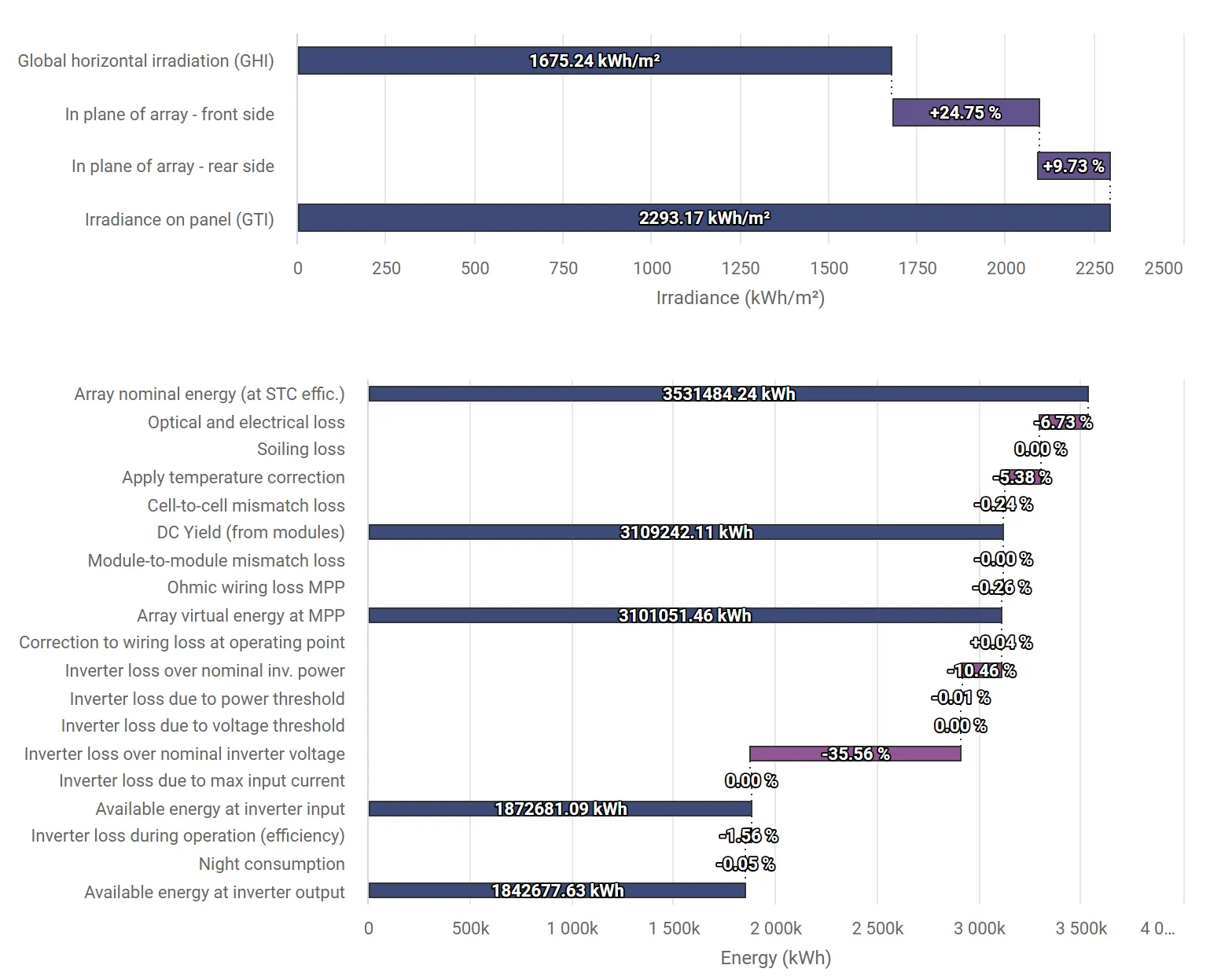Figure 6 – SunSolve waterfall loss chart example.

---

Time Series Data Output

The time series output interface allows users to download detailed, time-resolved simulation data for any SunSolve Yield project. Results can be exported for periods ranging from a single day to a full year, and are compatible with external analysis tools such as PVSyst.

Each dataset includes both input conditions and simulation outputs, covering all key domains — solar geometry, atmospheric parameters, module and string-level performance, and array-level electrical outputs. Users can select between different aggregation levels (module, string, or array) and enable or exclude additional filters such as nighttime data or error rows.

Available variables include solar position (zenith, azimuth, elevation), irradiance components (GHI, DHI, DNI), weather inputs (temperature, wind, humidity), and detailed electrical metrics such as Pmp, Vmp, Imp, Isc, temperature losses, and mismatch effects. The output also reports DC and AC power, conversion losses, and clipping conditions, providing a complete view of system behavior over time.

---

Hourly heat maps of per cell generation

SunSolve Yield can generate hourly heat maps that visualise the distribution of absorbed light across every cell within a PV module for any selected time step. These maps can be separated into front and rear surfaces and into direct and diffuse light components, providing a detailed spatial view of module illumination. By highlighting non-uniform absorption patterns, the heat maps help users identify sources of optical loss and understand conditions that contribute to electrical mismatch or reduced module performance.

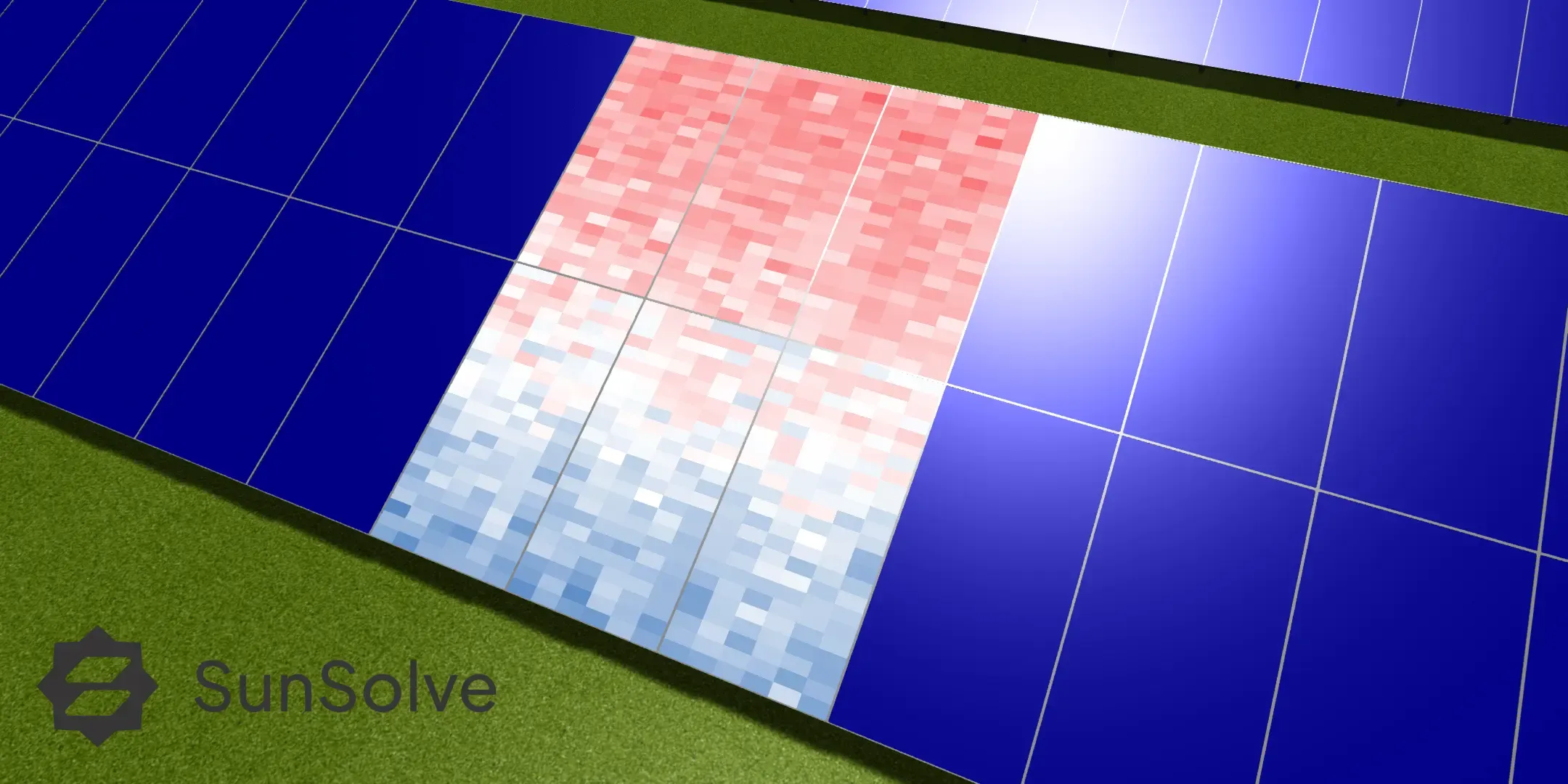
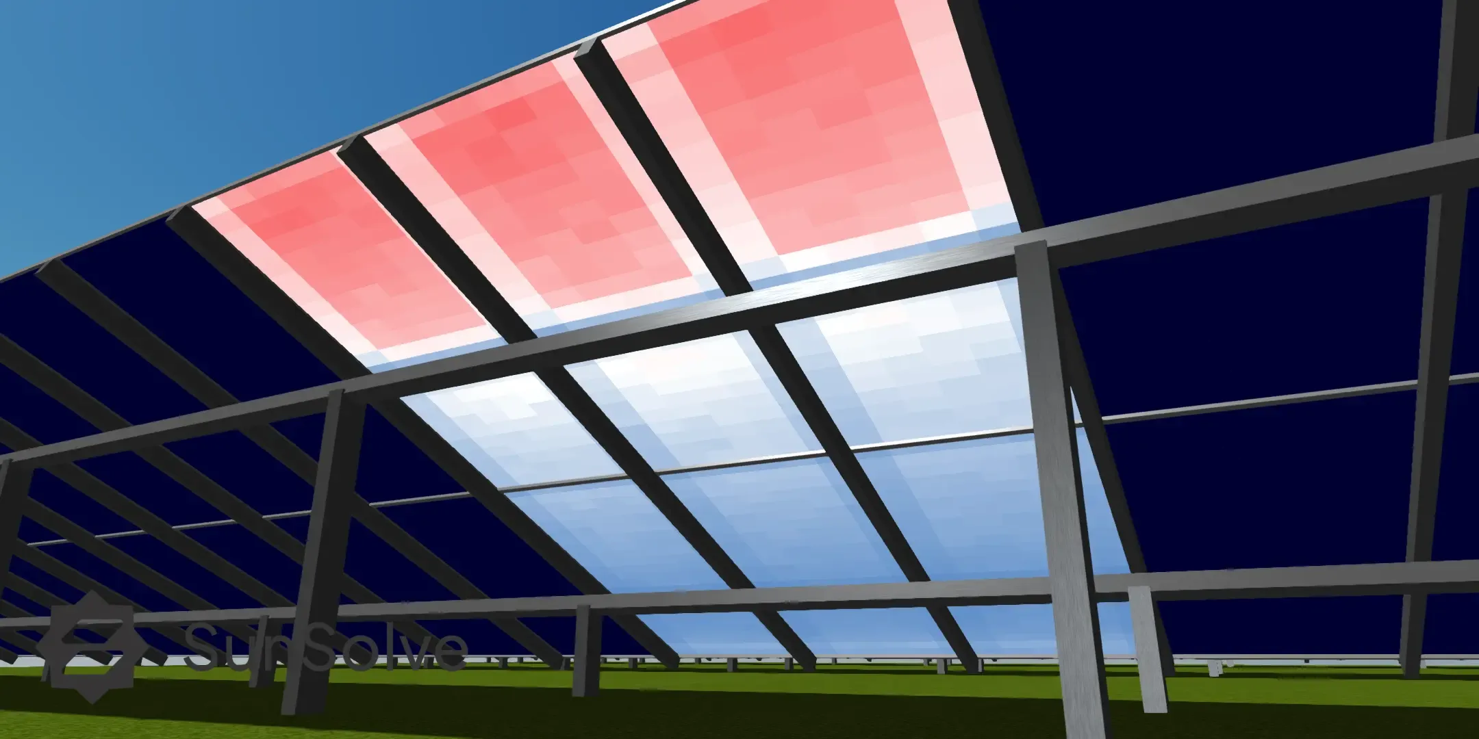Figure 7 – Example heat map showing front (upper) and rear (lower) absorption distribution across PV modules in a bifacial fixed tilt system.

---

Full Spectral Solving

The SunSolve engine fully accounts for the spectral dependence of incident irradiance, considering the effects of atmospheric conditions, geographic location, and time of day for both direct and diffuse components of sunlight. It also models the spectral characteristics of reflections from the ground and surrounding structures, ensuring that secondary illumination is represented accurately. SunSolve includes a comprehensive database of wavelength-dependent reflectance data for a wide range of common materials.

The optical modeling of PV modules likewise incorporates spectral effects, including the spectrally dependent incidence angle modifier (IAM) from anti-reflection coatings, as well as the dispersion properties of glass, encapsulants, and other materials within the module stack. In advanced configurations, SunSolve can even simulate the impact of spectral variation on sub-cell mismatch within tandem or multi-junction solar modules.

Spectral dependence is enabled by default, with carefully validated parameter sets derived from years of PV system and module modeling experience. For users developing novel technologies, custom spectral input data can be defined, and SunSolve engineers can assist in creating highly detailed wavelength-dependent material or layer models.

Accurately accounting for the spectral composition of sunlight is essential for reliable energy-yield prediction in all photovoltaic technologies. Although spectral variation is most pronounced in two-terminal tandem (2TT) devices, it also affects crystalline-silicon and other single-junction modules, particularly under atmospheres that shift the balance between blue and red wavelengths. Because the solar spectrum changes continuously with time, season, and atmospheric conditions, a module’s conversion efficiency can deviate significantly from its rated AM1.5g performance. These deviations—expressed through the spectral correction factor (fλ)—can influence annual energy yield by several percent, even for silicon systems, and by much more for tandem architectures. Incorporating spectral effects ensures that yield simulations capture current mismatch, bifacial gain, and real-world performance losses with high physical fidelity.

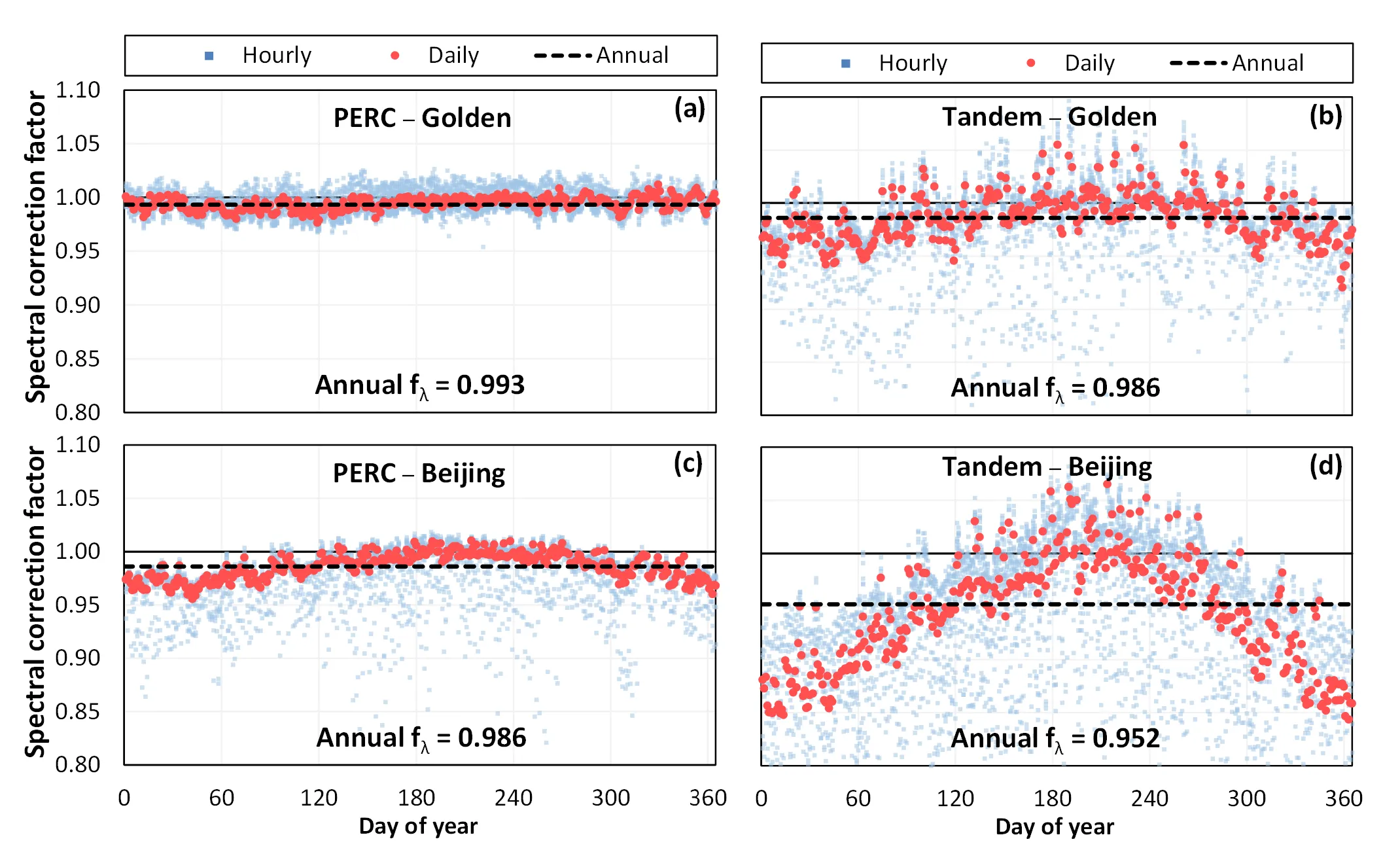
Figure 8 – Spectral correction factor calculated using SunSolve for different module technologies at different locations.

---

Advanced Optical, Thermal, and Electrical Simulations

The SunSolve engine is fully physics-based and consists of three tightly integrated components:

1. An advanced optical solver, built on forward ray tracing and parallel computation for exceptional speed and accuracy.
2. A robust thermal model that extends traditional approaches to deliver measurable improvements in module temperature prediction.
3. A SPICE-based electrical model capable of rapidly calculating cell-, module-, and string-level IV curves at every time step.

Together, these models allow SunSolve Yield to reproduce the complete physical behavior of a photovoltaic system — from photon absorption to AC power output — with industry-leading precision.

Optical Solving

The optical engine in SunSolve combines forward ray tracing with thin-film optics to predict the optical performance of complex PV systems. It incorporates years of specialised model development tailored to the photovoltaic industry, including advanced representations of surface textures, scattering, metallisation geometries, coatings, and other optical features.

As described in earlier sections, the optical solver accounts for wavelength-dependent behaviour across the full solar spectrum. By default, the spectral response from 300 nm to 1200 nm is resolved in 20 nm increments, capturing the detailed spectral effects essential for accurate performance prediction.

SunSolve Yield also supports simplified optical models compatible with other software, such as PVSyst, enabling the import of basic module definitions into advanced SunSolve scenes. This interoperability allows users to benchmark results between simplified and high-fidelity models, and to derive calibrated inputs that align conventional tools with SunSolve’s physically accurate simulations.

Thermal Model

The thermal model in SunSolve solves the complete energy balance between absorbed light, generated electrical power, and heat loss to the environment. Building upon the widely used Faiman model, it improves predictive accuracy through a detailed treatment of environmental and geometric effects.

The model accounts for sky, ground, and ambient temperatures, as well as transient thermal behaviour, where module temperature depends on its prior state — a critical capability for simulations with time steps shorter than 15 minutes. For highly calibrated sites, the model can also incorporate wind speed, direction, and their interaction with module tilt, providing realistic temperature dynamics for both fixed and tracking systems.

Electrical model

The electrical model begins at the cell level, where each solar cell is represented by an equivalent circuit that converts optical absorption and cell temperature into an IV curve. These cell circuits are then connected to form a module, incorporating key features such as bypass diodes and resistive interconnects.

Modules are combined in series and parallel to form complete strings and arrays, which are in turn connected to an inverter. The resulting array IV curve — adjusted for wiring losses — determines the system’s operating point and the corresponding AC output.

SunSolve supports all modern solar cell technologies, including PERC, HJT, and back-contact devices. It can also simulate two-terminal (2T) and four-terminal (4T) tandem architectures, enabling engineers and researchers to evaluate emerging technologies within realistic system contexts.

---

Integration with Industry Standards

SunSolve Yield is designed to operate seamlessly within the broader photovoltaic (PV) simulation ecosystem. It supports the workflows, data formats, and interoperability standards commonly used by researchers and engineers across the industry.

PVSyst Integration

SunSolve Yield includes validated workflows — published in PV Lighthouse white papers — for determining correction factors that can be applied as inputs in PVsyst and other energy-yield tools. These factors include:

• Shading and transmission factors for rear side view factor models
• Spectral mismatch corrections (fλ)
• Bifacial gain and mismatch factors
• Angular loss and albedo interaction coefficient
• Module temperature and view-factor adjustments

These parameters allow users to translate high-fidelity, physics-based SunSolve simulations into simplified correction factors suitable for use in conventional bankability models, ensuring consistency between advanced optical simulations and system-level yield predictions.

Parameter calculation is fully automated and integrated within the user interface.

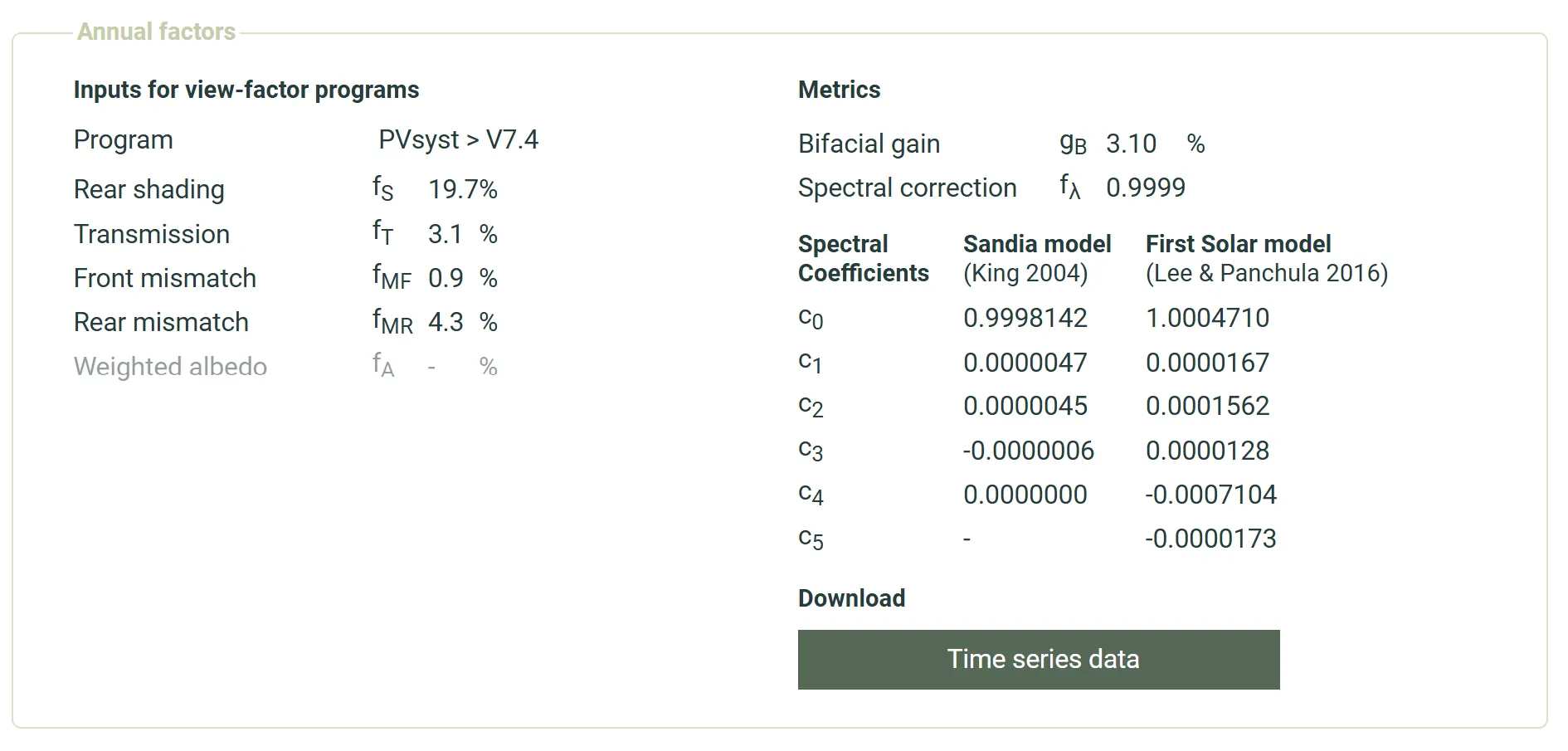
Figure 9 – Example of SunSolve Yield analysis output used to derive bifacial correction factors for PVSyst integration.

Weather Data Compatibility

SunSolve Yield can load weather and irradiance data from a wide range of sources, including:

• TMY3, SolarAnywhere, Solargis, Solcast, and Vaisala file formats
• On-site measured datasets in CSV or other custom time-series formats
• Integration with PVGIS and other cloud-based meteorological services for regional datasets

Weather inputs such as GHI, DNI, DHI, ambient temperature, and wind speed form the fundamental description of the simulation site. These can be extended with parameters such as precipitable water vapour, relative humidity, atmospheric pressure, ozone, and aerosol optical density to enhance site-specific spectral accuracy.

SunSolve Yield supports any time-step length, including 5-minute, 15-minute, or hourly intervals, allowing both research-grade and operational-scale simulations to be performed with required time precision.

Model Interoperability and Outputs

SunSolve Yield exports results in widely recognised formats for downstream analysis, enabling interoperability with:

• PVsyst, SAM, and other yield modeling tools
• CSV and Excel-compatible time-series data for custom analytics
• JSON-based structured outputs for automation and scripting workflows

All outputs follow industry conventions for parameter naming, units, and time alignment, simplifying comparison and integration with existing pipelines.

Validation and Standardisation

SunSolve Yield’s models and correction workflows have been benchmarked against published standards and validated in collaboration with academic and industrial partners. This alignment ensures that the software not only provides high physical accuracy but also produces results that are traceable to standard PV performance metrics.

Access and Integration

Access to the SunSolve Yield solver can be achieved either through the web-based portal or directly via the API, allowing flexible integration into existing workflows.

The web interface is ideal for interactive simulation setup, visualisation, and analysis, while the API provides direct programmatic access for automation, batch processing, or coupling with other simulation environments such as PVSyst or custom research pipelines.

---