Insolation

At each time step, SunSolve computes

• the sun’s position, i.e., the solar zenith and azimuth;
• the solar spectrum for direct and diffuse light; and
• the fraction of sunlight ascribed to the beam and isotropic components.

This section describes the models used for these computations. The table below summarises the default models used in SunSolve Yield to compute the insolation.

Parameter	Model	Reference
AM0 spectrum	IEC standard	[IEC2008]
Clear-sky spectra	SPECTRL2	[Bird1986]
Cloudy-sky spectra	Ernst	[Ernst2016]
Solar position	Reda and Andreas	[Reda2004]
Air mass	Karsten	[Karsten1989]
Diffuse-sky distribution	Perez 1990	[Perez1990]
Earth–Sun correction factor		[Bird1986]
Equation of time		[Reno2012]

Solar position

General definitions

• Solar zenith and solar azimuth are defined with respect to the centre of the sun.

• Solar zenith is defined as 0° when the sun is directly overhead.

• Solar azimuth is defined clockwise from north, i.e., north = 0°, east = 90°, south = 180°, west = 270°.

• Sunrise and sunset are defined as the time to the nearest second when the zenith angle is 90°.

Options for setting the solar position

The user can either

1. set the solar position to values in a weather file, or

2. allow SunSolve to calculate the solar position from the location of the system, the date and the time.

For the first option, the user loads a weather file that contains the solar position at each time step. The position can be defined with either the solar zenith or the sun height (i.e., 0° when at the horizon and 90° when directly overhead), and with the solar azimuth defined as either clockwise from north or with various other definitions that are found in different weather services.¹

Irrespective of the inputs, SunSolve’s outputs for solar position are always the solar zenith and azimuth, as defined above under “general definitions”.

For the second option, the user selects an algorithm for the solar vector (unaffected by the atmosphere), and atmospheric refraction.

Solar-vector models

There are seven solar-vector models. The references contain the relevant equations:

1. Reda and Andreas 2004 [Reda2004].

2. Blanco–Murial 2001 [Blanco2001].

3. Michalsky 1988 [Michalsky1988].

4. Walraven 1979 [Walraven1978].

5. Spencer 1971, our implementation from [Reno2012]

6. ASCE (2012), our implementation from [Reno2012]

7. PVSyst, as described in the PVSyst documentation (as of Apr-2023).

The most sophisticated of the solar-vector models is the Reda and Andreas 2004 model. It implements an algorithm developed by Meeus in 1998 to compute the zenith and azimuth to within ±0.0003° between the years 2000 BCE and 6000 CE. The implementation within SunSolve is modified to exclude refraction so that its impact can be computed separately. This model has been the default in SunSolve since May 2023.

The second-most complicated model is that of Blanco–Muriel 2001, which computes the solar vector to within 0.5 minutes of arc between 1999 and 2015. This was the default in SunSolve until May 2023.

The other models are simpler and less accurate, they are included in SunSolve to allow comparisons to historical solar-vector algorithms and other software.

Atmospheric refraction models

SunSolve has three options for atmospheric refraction:

1. None, i.e., no correction in solar position due to refraction is applied.

2. Reda and Andreas (2004) [Reda2004].

3. Zimmerman (1981) [Zimmerman1981].

The Reda and Andreas model is the most accurate. It requires inputs for the altitude, air pressure and ambient temperature. These inputs can be loaded with the weather, but if not, they are assumed to be 0 m, 1013.3 mbar and 25 °C.²

Solar position for a time interval

SunSolve computes the yield for a series of time intervals and sums them to determine the total yield. This is described in the previous section.

For most time intervals, the solar position is computed at the mid-point of that interval. For example, if SunSolve is computing the yield for the interval 10–11 am, it calculates the solar position at 10:30 am.

Exceptions arise for any interval that includes sunrise or sunset. In that case, the solar position is calculated at the mid-point of the daylight period.³ For example, when sunrise is at 6:30 am, the solar position for the interval 6–7 am would be calculated at 6:45 am. And when sunset is at 5:40 pm, the solar position for the interval 5–6 pm would be calculated at 5:20 pm.

Solar spectra

The direct and diffuse spectra are calculated at every timestep as follows:

1. The extra-terrestrial spectrum is calculated.

2. The direct and diffuse spectra for clear-sky conditions are calculated.

3. The direct and diffuse spectra are modified for cloud.

4. The spectral intensity of the direct and diffuse spectra are scaled so that the integrated irradiance equals the desired DNI and DHI.

5. The spectral irradiance is converted into photon flux.

We determine Steps 1–4 with a wavelength range of 280–4000 nm and an interval of 5 nm (744 wavelength bins). This range covers more than 99% of the intensity of the solar spectra. In Step 5, the range is reduced to 300–1200 nm and the interval is increased to 20 nm (46 bins). This range covers just the active region of a silicon semiconductor. The ray tracing is conducted for all 46 wavelength bins.

Extra-terrestrial spectrum, AM0

The extra-terrestrial spectrum defines the solar spectrum reaching Earth’s outer atmosphere. SunSolve uses the AM0 spectrum from the IEC standard, [IEC2008], which defines this spectrum when the Earth is at its average distance from the Sun.

SunSolve then multiplies the spectral intensity by the ‘Earth–Sun factor’ at each time interval. This factor is determined from Equations 3 and 4 in [Bird1986], and accounts for the elliptical nature of Earth’s orbit. (It is unity around the 3rd of April and the 1st of October.)

Clear-sky spectra

The SPCTRAL2 algorithm [Bird1986] is used to determine the wavelength-dependent transmission of direct and diffuse light through the Earth’s atmosphere on a clear day, which is then used to convert the AM0 spectrum into the direct and diffuse spectra.

As well as the time and global location, the algorithm requires six inputs: air mass, far-field albedo, and four parameters that define the atmosphere: air pressure, turbidity at 500 nm, precipitable water vapour concentration, and ozone concentration.

The most influential of the six inputs is the air mass AM, calculated from the solar zenith θs,

$$AM = \begin{cases} \frac{1}{\cos \theta_s + 0.50572 \times (96.07995 - \theta_s)^{-1.6364}}, & \theta_s \leq 91.8° \\ 64.8, & \theta_s > 91.8° \end{cases}$$

For θs ≤ 91.8°, the equation is the widely used parameterisation of Karsten and Young [Kasten1989]. In SunSolve, we limit the calculations to θs < 91.8° to prevent crashes.⁴

The remaining five inputs are loaded with the weather, or if they are not available, default values are applied. The table below lists those inputs, the default values⁵ and possible sources for determining the inputs for a particular location. The default values are those used to generate the AM1.5g spectrum when the air mass is 1.5. Note that the albedo contributes only to the spectral intensity of the diffuse light, since light can reflect from the ground to the sky and then back again to the ground; it is assumed constant with wavelength in SPCTRAL2.⁶

Atmospheric inputs used in simulations, listed in order of how much they affect the solar spectra. The NASA data can be sourced from the Giovani website

Property	Units	AM1.5g default	SunSolve7	Possible sources
Precipitable water vapour	cm	1.416	Loaded in weather	TMY weather file (Meteonorm, SolarGIS)
Turbidity at 500 nm		0.084	Loaded in weather	NASA: Time Series, Area-Averaged of Aerosol Optical Depth 500 nm daily 1 deg.
Ozone	DU	343.8	Loaded in weather	NASA: Time Series, Area-Averaged of Ozone Total Column (TOMS-like) daily 1 deg.
Atmospheric pressure	mbar	1013.25	Loaded in weather	TMY weather file (Meteonorm, SolarGIS)
Far-field albedo		10%	Loaded in weather	Site measurement, TMY weather file, Satellite data.

See impact of atmosphere on spectrum for plots of how these factors impact the direct spectrum.

Cloudy-sky spectra

To account for clouds, the clear-sky spectra are adjusted in a manner like that described by [Ernst2016].⁸ At each timestep, the procedure is as follows:

1. The direct (beam) $I_{B\text{ clear}}(\lambda)$, diffuse $I_{D\text{ clear}}(\lambda)$ and global $I_{G\text{ clear}}(\lambda)$ irradiances are determined for clear-sky conditions using SPECTRL2 over the range 280 ≤ λ ≤ 4000 nm in steps of 5 nm.

2. The direct (beam) spectrum for cloudy conditions equals the clear-sky direct spectrum scaled to give the measured DNI,

   $$I_{B \text{ cloudy}}(\lambda) = I_{B \text{ clear}}(\lambda) \cdot \frac{DNI}{\int_{280}^{4000 \text{ nm}} I_{B \text{ clear}}(\lambda) d\lambda}$$

   I.e., the relative spectrum of the direct light is the same whether clear or cloudy.

3. A cloud-opacity factor OF is calculated. It relates to the direct-normal insolation DNI taken from the weather file divided by the DNI of the clear-sky spectrum (i.e., $I_{B\text{ clear}}(\lambda)$ of Step 1):

   $$OF = 1 - \frac{DNI}{DNI_{\text{clear}}} = 1 - \frac{DNI}{\int_{280}^{4000 \text{ nm}} I_{B \text{ clear}}(\lambda) d\lambda}$$

   and thus, OF quantifies the fraction of direct light that does not penetrate the clouds. Note that if $DNI > DNI_{\text{clear}}$, we override this equation and set OF = 0.

4. The unscaled diffuse spectrum for cloudy conditions is given by

   $$S_{D \text{ cloudy}}(\lambda) = I_{D \text{ clear}}(\lambda) + OF \cdot I_{B \text{ clear}}(\lambda) \cdot \cos(\theta_z),$$

   i.e., the clear-sky diffuse spectrum plus the clear-sky direct spectrum that does not penetrate the clouds.

5. The diffuse spectrum for cloudy conditions is then scaled to give the DHI of the weather file

   $$I_{D \text{ cloudy}}(\lambda) = S_{D \text{ cloudy}}(\lambda) \cdot \frac{DHI}{\int_{280}^{4000 \text{ nm}} S_{D \text{ cloudy}}(\lambda) d\lambda}.$$

By taking this approach, we assume that (i) the direct spectra on a cloudy day are the same as on a sunny day except attenuated, and (ii) the diffuse spectra are the same as on a sunny day except attenuated and combined with the global spectra.

In effect, this approach treats the clouds as neutral-density filters and neutral-density scatterers.

In reality, the transmission through clouds tends to decrease with wavelength. PV Lighthouse is in the process of permitting SunSolve users to select a cloudy-sky spectral model that takes this into account. A cloudy-sky spectral model is available from NREL’s FARMS-NIT program but it does not currently distinguish between direct and diffuse cloudy-sky spectra (Mar-2025).

Sky distribution of diffuse light

SunSolve Yield provides three options for the sky distribution of diffuse light: (1) isotropic, (2) the Hay-Davies model and, (3) the Perez model. In the first case the angular distribution of the light is unchanged based on weather conditions and always assumed uniform from all points in the sky. In the Hay-Davies and Perez models the amount of cloud is used to assign some fraction of the diffuse irradiance into a circumsolar area around the location of the sun. More cloud results in more isotropic conditions and clearer days result in more circumsolar component. The angle of the circumsolar light is assumed to be equal to the solar zenith (i.e. it appears to come directly from the sun). In the case of the Perez model there are several variations that have been implemented.

Hay-Davies model

The Hay-Davies model is applied at each timestep using the procedure:

1. The sky clearness index ($K_b$) is calculated using the following equation:

   $$K_b = \frac{I_{\text{direct,perp}}}{I_0 \times d}$$

   where $I_{\text{direct,perp}}$ is the intensity of the DNI, $I_0$ is the extra-terrestrial intensity of sunlight 1367 W/m2, and d is the Earth-Sun correction factor calculated using equation Eq. 2 of [Bird1986]:

   $$d = 1.00011 + 0.034221 \times \cos \psi + 0.00128 \times \sin \psi + 0.000719 \times \cos 2\psi + 0.000077 \times \sin 2\psi$$

   and ψ is the day in radians calculated from [Bird1986] using:

   $$\psi = 2\pi \times \frac{(\text{DayOfYear} - 1)}{\text{DaysInYear}}$$

2. The value of Kb is then used to adjust the direct and diffuse intensity of light as follows:

   $$J_{\text{ph,direct normal}}(\lambda) = J_{\text{ph,direct normal}}(\lambda) + \frac{K_b \times J_{\text{ph,diffuse horizontal}}(\lambda)}{\cos \theta_s}$$ $$J_{\text{ph,diffuse horizontal}}(\lambda) = (1 - K_b) \times J_{\text{ph,diffuse horizontal}}(\lambda)$$ $$DNI = DNI + \frac{K_b \times DHI}{\cos \theta_s}$$ $$DHI = DHI - K_b \times DHI$$

   Where $θ_S$ is the solar zenith.

Perez models

There are three implementations of the Perez model included in SunSolve.

• Perez (1987) - an earlier version of the Perez model based on [Perez1987].

• Perez (1990) - a newer version of the Perez model based on [Perez1990]. This is the most used Perez model.

• Perez (SAM) - a version of Perez 1990 adapted by NREL for use in the System Advisory Model tool [Gilman2018].

The Perez model (Eq 9 in [Perez1990], Eq 12 in [Loutzenhiser2007]) for the diffuse irradiance on an inclined plane is

$$G_{SF\_dif} = DHI \cdot \left[(1 - F_1) \cdot \frac{1 + \cos \beta}{2} + F_1 \frac{a}{b} + F_2 \sin \beta\right], \tag{1}$$

where $F_1$ and $F_2$ are circumsolar and horizontal brightness coefficients, and where a and b are given by⁹

$$a = \max(0, \cos \theta_i) \tag{2}$$

and¹⁰

$$b = \max(0.087, \cos \theta_s), \tag{3}$$

The brightness coefficients are given by¹¹

$$F_1 = f_{11} + f_{12}\Delta + f_{13}\theta_s \tag{4}$$

and

$$F_2 = f_{21} + f_{22}\Delta + f_{23}\theta_s \tag{5}$$

where

$$\Delta = AM \cdot \frac{DHI}{DNI_0}, \tag{6}$$

and where AM is the relative optical airmass.¹²

The f coefficients were derived from a statistical analysis of empirical data for specific locations and they depend on the sky clearness ε,¹³

$$\varepsilon = \frac{\frac{DHI + DNI}{DHI} + 1.041 \cdot \theta_s^3}{1 + 1.041 \cdot \theta_s^3}, \tag{7}$$

Hence, on an overcast day with no direct light, DNI = 0 and the clearness ε = 1; on clearer days, DNI increases, and ε increases above unity.

Different values of f have been derived in [Perez1987] and [Perez1990] and they depend on different bounds for ε. Table V and Table VI give those values.

Table V: Clearness bins.

ε category	Upper Bound
	[Perez1987]	[Perez1990]
1 – overcast	1.056	1.065
2	1.253	1.230
3	1.586	1.500
4	2.134	1.950
5	3.230	2.800
6	5.980	4.500
7	10.080	6.200
8 – clear	–	–

Table VI: Values for f coefficients from (a) [Perez1987] and (b) [Perez1990]. Here we use the irradiance coefficients rather than the illuminance coefficients.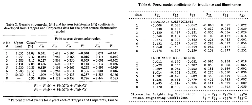

The Perez model is applied at each timestep using the procedure:

1. Sky clearness (ε) is determined using equation (7).

2. The values for the Perez coefficients are calculated using Table VI (based on the selected Perez model). Linear interpolation is applied to determine the F values for any value of ε. Note that the SAM model uses the Perez1990 coefficients.

3. Sky brightness (Δ) is determined using equation (6)

4. Brightness coefficients for circumsolar (F1) and horizon brightening (F2) are calculated using equations (4) and (5).

5. The value of F1 is then used to adjust the direct and diffuse intensity of light as follows:

   $$J_{ph,direct\ normal}(\lambda) = J_{ph,direct\ normal}(\lambda) + \frac{F_1 \times J_{ph,diffuse\ horizontal}(\lambda)}{\max(0.087, \cos\theta_s)}$$ $$J_{ph,diffuse\ horizontal}(\lambda) = (1 - F_1) \times J_{ph,diffuse\ horizontal}(\lambda)$$ $$DNI = DNI + \frac{F_1 \times DHI}{\max(0.087, \cos\theta_s)}$$ $$DHI = DHI - F_1 \times DHI$$

   Where $θ_S$ is the solar zenith.

6. The horizon brightening is assumed to have never interacted with a panel since the simulation field is infinitely large and the incidence angle of that component is parallel to the flat ground. Thus, some fraction of the light is removed from the scene.

---

Footnotes

1. SunSolve automatically attempts to detect the Azimuth definition by comparing the loaded values with a calculation of the sun position, from this an adjustment is applied to map the azimuth onto the SunSolve definition. ↩

2. The calculation of the solar matrix (see Optics: Solar arcs) assumes these default values irrespective of the user inputs. The assumption has negligible impact on SunSolve’s results because the solar matrix is interpolated using the correct solar position (i.e., without the assumption). ↩

3. Although these time intervals contain a partial period of sunlight, the assumed GHI is for a full period. Thus, SunSolve multiplies the module power by the full period when computing the yield.. ↩

4. Note that solar zenith angles greater than 90° are anyway considered night and do not make use of air mass. ↩

5. These defaults were developed decades ago by NREL from measurements at Golden, Colorado. They should not be expected to apply at every location globally. ↩

6. Note that this albedo value is the ‘far-field’ albedo (defined as part of the weather file for the location) and is not the same as the wavelength dependent albedo that is included during the ray-tracing of the unit-system. ↩

7. Atmospheric inputs default to the AM1.5g values if not defined by the user for a specific location. ↩

8. While we follow the general approach of Ernst et al., the actual equations we apply differ. There appears to be an error in their Eq 7 (omission of cosθz), the combination of Eqs 5, 7 and 8 is not, to our mind, entirely logical, and the optical factor (Eq 5) is (ρ – ρclear)/(1 – ρclear), where ρ = DHI/GHI, which is equivalent to OF = 1 – (DNI/GHI)/(DNIclear/GHIclear) rather than 1 – DNI/DNIclear. We do, however, capture the purpose of their approach (as communicated by Ernst) rather than the exact equations. That is, (i) the relative direct spectrum is the same on clear and cloudy days, (ii) the relative diffuse spectrum is the clear-sky diffuse spectrum PLUS whatever clear-sky direct spectrum did not pass through the clouds, and (iii) the spectra are scaled to ensure their integral equals the DNI and DHI in the weather file. (It is point (ii) that differs from Eqs 5, 7 and 8.) ↩

9. Notice that a/b = cosθi/cosθs except that θi and θs are limited to θi ≤ 90° and θs ≤ 85°. The limitation on a ensures that the circumsolar is zero when the sun is behind the panel. ↩

10. In [Loutzenhiser2007], they use b = max(85°, cosθs), which is not quite the same thing. ↩

11. In the following equations, θs is in radians. Loutzenhiser2007 forces F1 ≥ 0 but Perez1990 doesn’t appear to do so. ↩

12. Perez et al. cite Kasten1966 for their air mass equation. SunSolve applies the same equation. ↩

13. In the first paper on the Perez model [Perez1990], the sky clearness is ε = (DHI + DNI) / DHI. ↩