Fundamental optics

SunSolve ray tracing is based on thick optical slabs (which are treated as being optically incoherent) with complex optical interfaces where those slabs meet. There are two types of optical interfaces: (1) Fresnel and (2) Basic reflectors.

In the first type (Fresnel) the percentage chance of reflection, absorption or transmission is determined from fundamental physics based on the optical properties of the materials either side of the interface, and any thin films at the interface. Solving of the optics is based on the Fresnel equations, uses an adapted version of the transfer matrix method and accounts for polarization of the light. In the second case (basic reflector) these percentages are set as an input to the program. They are typically determined based on experimental measurement.

Optical interfaces may also include a morphology (commonly referred to as texture) and additional scattering.

The table below provides a summary of the optical models applied to the interfaces.

Parameter	Model	Notes	Reference
Absorption in material	Lambert-Beer law		-
Reflection, absorption, transmission at interface	Fresnel	Applied for Fresnel interfaces	-
Ray direction	Snell’s law
Scattering fraction	Fixed	User defines %	-
Scattering fraction	Scalar scattering-model		[Carniglia1979] [Dominé2010]
Scattering distribution	Lambertian
Scattering distribution	Phong	Modified to account for transmission	[Phong1975] [Schümacher1994]

For a more detailed explanation of the physics upon which the SunSolve engine is based the reader is referred to the online lecture series by Pietro Altermatt.

Available here: https://pvlighthouse.com.au/cms/lectures/altermatt/optics/

Fresnel interfaces

An optical Fresnel interface is solved using fundamental optical equations. This uses the wavelength dependent refractive index of the material slabs on either side, combined with any thin films present. This solving is used to determine the percentage chance the ray with be reflected, transmitted, or absorbed at the interface.

Basic reflectors

An optical interface that has been defined as a reflector does not apply any complex optical interface solving. Instead, it applies a look-up table that defines the fraction of incident light that is reflected, absorbed, or transmitted. This table may be defined as being wavelength dependent.

Surfaces of modules have additional options for the application of the basic reflector. These include an angular dependence to the reflection, absorption, and transmission. More detail on this is provided in section 6.1.

Texture models

The surface morphology (i.e., the texture) of an interface can be set to one of several options. Images of the non-planar options are shown below, where the image depicts the feature that is repeated in the x and y directions over the entire interface. The user sets the angle ω, and the height h or width of the surface feature.

Note that (i) a V groove extends across the entire x or y expanse of the interface, depending on whether the user selects an x or y orientation; and (ii) a corner cube [Van2015] has a fixed ω and a regular hexagonal unit cell.

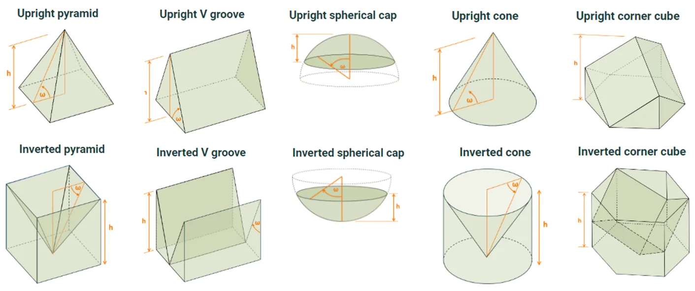Non-planar surface morphology options, shown as unit blocks.

Random morphologies

The program provides the option to select either ‘random’ or ‘regular’ surface morphologies (i.e., texture). This helps simulate, for example, the ‘randomly’ oriented pyramids that cover the front surface of industrial monocrystalline silicon wafers, or the ‘regular’ inverted pyramids that have been employed in high-efficiency laboratory PERL solar cells.

The figure below demonstrates how ‘random’ morphologies affect the propagation of rays during ray tracing. The simplest geometrical feature of a morphology (e.g., a pyramid or a groove) is bounded by the planes of its unit cell. A ray that intersects the wall of a unit cell is propagated into a neighbouring unit cell, whereas a ray that intersects the floor (or ceiling) of a unit cell is propagated into the layer below (or above) the feature. This might, for example, be the propagation of a ray from the textured region of a wafer to the bulk of the wafer.

The images below show how this propagation is achieved when a ‘random’ morphology is selected. They depict a ray intersecting (i) a wall and (ii) the floor of a unit cell. When the ray intersects one of these boundary planes, it is assigned a new random location on that boundary, and then the ray is propagated into the neighbouring unit cell (or layer) via the same location on the common boundary and with the same propagation angle. Thus, the features are not rotated but merely translated with respect to one another.

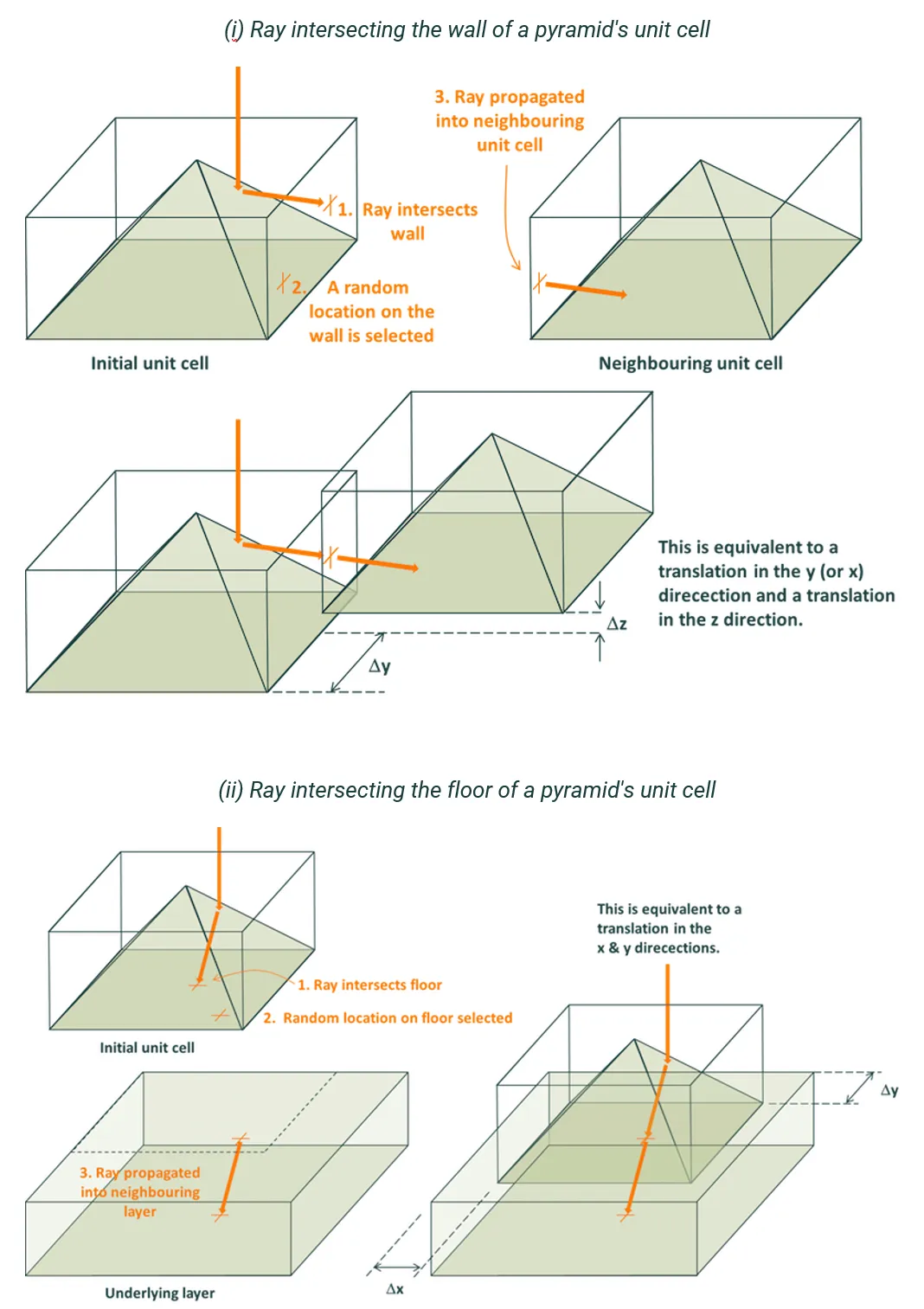Ray tracing algorithm used to simulate unit-textures with random morphology.

Scattering models

All types of interfaces can have additional scattering. Scattering is defined with two selections: (1) distribution (i.e., the angular distribution of scattered light) and (2) fraction (what percentage of the light is scattered). In the case of a textured surfaces scattering is defined as occurring on the facets of the texture. When scattering is imposed at a surface, SunSolve randomises the polarisation of the ray after it interacts with the surface.

Scattering distribution

Optical scattering is implemented by one of three models: ‘no scattering’, ‘Lambertian scattering’ or ‘Phong scattering’ [Phong75]. These models are represented by the diagrams below.

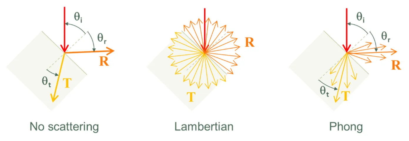Optical scattering models.

Whenever a ray intersects an interface, SunSolve first determines if the ray is reflected or transmitted using the stochastic approach described in Section 4.1. SunSolve then determines the new direction of the ray, where this direction depends on the scattering model. With no scattering, the ray’s new direction is determined by assuming that the interface is specular and hence the reflectance angle θr equals the incident angle θi and the transmitted angle θt is given by Snell’s law.

Lambertian scattering

With Lambertian scattering, the spherical-polar angles (θ and φ) that define the ray’s new direction are determined stochastically from

$$\theta = \cos^{-1} \left( \chi^{\frac{1}{2}} \right)$$

and

$$\phi = 2\pi\chi$$

where χ is a random number, 0 ≤ χ < 1, and where unique random numbers are generated to determine θ and φ. With infinitely many rays, these equations lead to Lambertian reflection (or transmission), whereby the light intensity per solid angle is uniform. Notice that the new ray direction is independent of θi.

Phong scattering

With Phong scattering, SunSolve determines the new direction as

$$\Delta\theta = \cos^{-1} \left( \chi^{\frac{1}{1+\alpha}} \right)$$

and

$$\phi = 2\pi\chi$$

where α is called the Phong exponent, and where Δθ is the difference between the new angle and the specular reflection, Δθ = θ – θr, or the specular transmittance, Δθ = θ – θt, depending on whether the ray is reflected or transmitted. This follows Schümacher’s implementation of the Phong model for stochastic ray tracing [Schümacher1994].

Thus, Phong scattering is identical to Lambertian scattering when α = 1 and θi = 0 (normal incidence), and it is identical to ‘no scattering’ when α is infinite—although α = 1,000,000 is high enough to emulate a specular surface. SunSolve limits α to 1 ≤ α ≤ 1,000,000.

The figure below shows how the probability function f(Δθ) = (cosΔθ)1+α depends on Δθ and α. Note: this is not the intensity function.

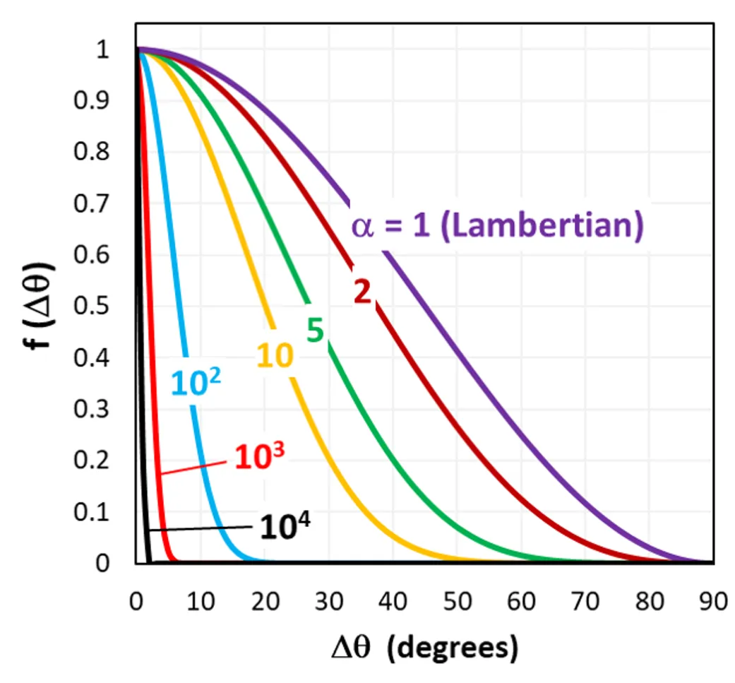Phong scattering, normalised angular distribution of the scatter angle shown for various values of the Phong exponent.

Notice from the above figure that Phong scattering can be used to simulate ‘focused’ scattering. For example, with α = 1000, the scattered light for a reflected ray will be approximately θ = θr ± 5°. This might be useful when simulating random pyramids whose base angles vary by ± 5°.

Scattering fraction

There are two approaches to computing the fraction of incident rays that are scattered.

The first approach is to set a constant scattering fraction Λ. This means that for each ray that interacts with the surface, Λ of these will be scattered by the chosen scattering model and the remainder will not be scattered. Thus, setting Λ = 0 will mean that there is no scattering, no matter what scattering model is selected.

The second approach is to apply the scalar scattering-model [Carniglia1979][Dominé2010]. With this model, the scattering fraction Λ is not constant but decreases with increasing wavelength. This fraction also depends on the incident angle, the refractive index of the materials and whether the ray is reflected or absorbed. This model is intended to approximate the response of a surface on which the scale of the geometric features is of a similar magnitude to the incoming wavelength of light (e.g., black silicon nano-texture).

For reflection,

$$\Lambda = 1 - exp \left[ -\left( \frac{2\pi}{\lambda} \cdot \sigma_{rms} \cdot 2 \cdot n_i \cdot \cos\theta_i \right)^2 \right]$$

and for transmission,

$$\Lambda = 1 - exp \left[ -\left( \frac{2\pi}{\lambda} \cdot \sigma_{rms} \cdot |n_i \cdot \cos\theta_i - n_t \cdot \cos\theta_t| \right)^2 \right]$$

where σrms is the root mean square roughness of the surface.

The figure below plots the scattering fraction as a function of wavelength and σrms for an incident medium of ni = 1.5 where the incident angle is either θi = 0° (solid) or 50° (dotted), as determined from the scalar-scattering model.

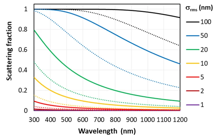Scattering fraction as a function of wavelength as defined by the scalar scattering implementation within SunSolve. Shown for various values of the input sigma which represents the root-mean-square roughness of the surface.

---