
How to simulate distributions in module power from measured cells
This guide outlines a step-by-step process to simulate the distribution in module output (, , , power) that will be caused by a distribution in cell performance.
The distributions in module output generated will include:
- the impact of distributions in per-cell current that occur as a result of cell location within the module (i.e. proximity to reflective white layers).
- stochastic noise from the ray tracer.
- optical gains and losses due to the module encapsulation process
- changes in series resistance that occur due to changing from single cell IV test probes into soldered, interconnected ribbons
- changes in the electrical model due to cell processing to integrate within a module (i.e. cell cutting)
The later part of the tutorial demonstrates alternative configurations of the SunSolve inputs to remove, study and minimise these effects.
Download example cell IV data
Section link: Download example cell IV dataThe example here is based on the SunSolve template for the TOPCon module and some synthetic solar cell data available for download below.
Download the sample cell file (2000 cells, CSV)
After learning from the tutorial, users should transition to using measured cell data and a well-calibrated SunSolve baseline model for the modules.
1. Create a new simulation with a module baseline model
Section link: 1. Create a new simulation with a module baseline model- From the SunSolve front page, click on the template group Modules.
- Click on the 144 half-cell TOPcon module template.
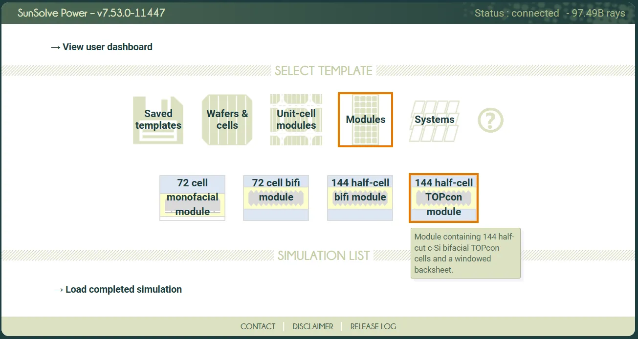
This will create a simulation with inputs that describe a generic example module. Alternatively at this point users can load their baseline model for a module.
2. Run the optical solver
Section link: 2. Run the optical solver- Click on the run triangle at the top of the screen to run the optical solver.

The ray tracing will now run, the baseline will be solved and the status should change to Done.
3. Define the base electrical circuit for the solar cell
Section link: 3. Define the base electrical circuit for the solar cell- Go to the Inputs > Cell tab.
- Set Ideality factor to 0.7.
- Switch on the diode by clicking on it in the circuit diagram.
- Uncheck the Incl. analytical Rs checkbox. We will not use the analytical grid solver in this example.
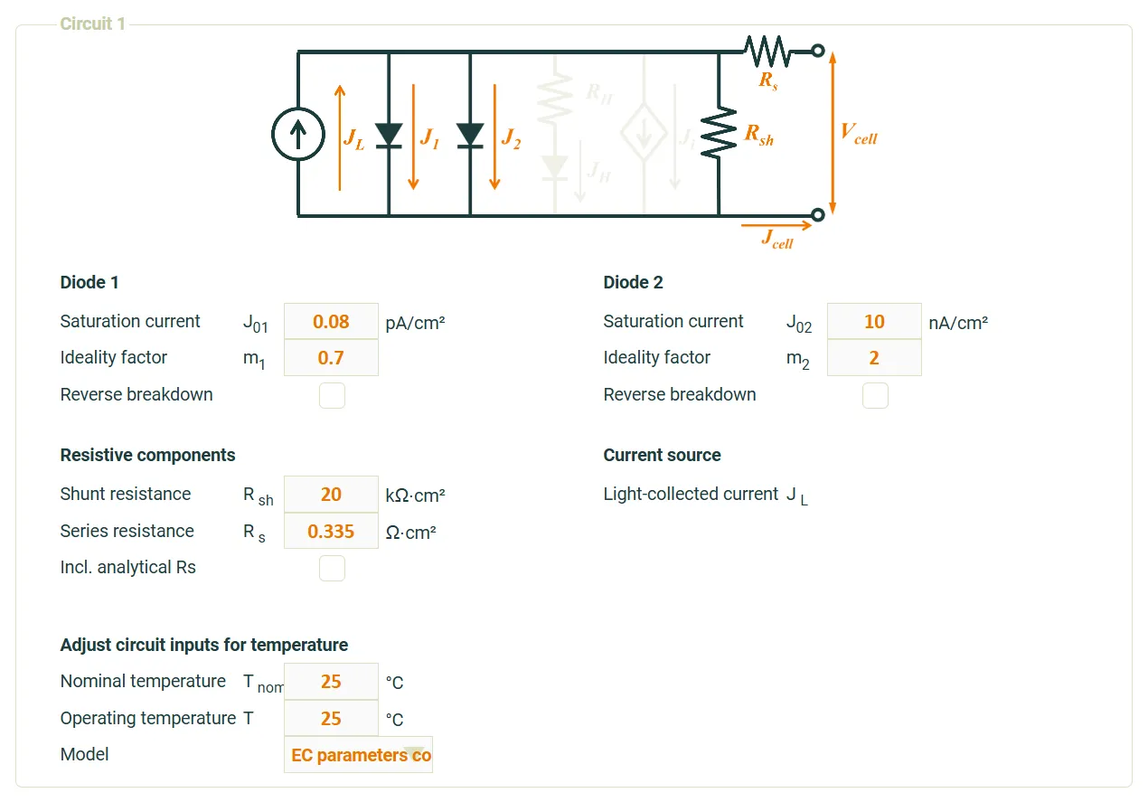
At this stage we are defining the base equivalent-circuit that we will use to simulate the solar cells. In practice this circuit may already closely align with the cells whose results we will shortly upload. Later we will modify it to account for changes that occur during module integration.
The most important part of this stage is to define which loss components we will include in the cells (, , , ) and what ideality factors to use in the diodes.
4. Load the measured cell results
Section link: 4. Load the measured cell results- Go to the Inputs > Modifiers tab.
- Select Module population.
- Set Modules to 2000.
- Select Measured cells (CSV).
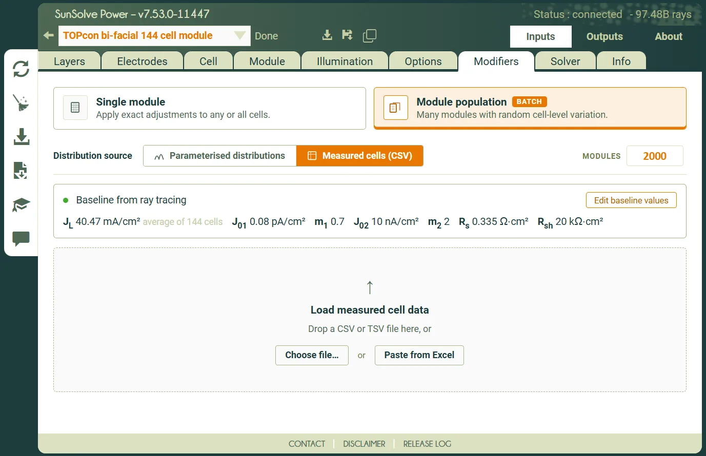
- Select Choose file… and then load the example cell IV data file.
- Set Enable binning to true.
- Set Binning by to IVBin_Imp.
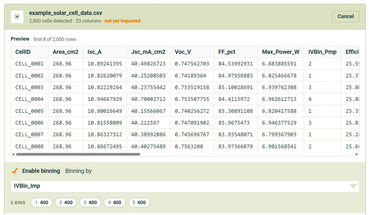
Note that the use of binning is optional. If the bins were allocated in the file it is worth loading them at this step as they can be switched off later if not required.
- Set Measured cell area to 268.96 cm². Note that this value was available in the cell IV file.

The inputs to SunSolve’s internal models are area-independent, so we require the actual area of the measured cell. That will allow the conversion from any area-dependent values (like ) into area-independent ones.
Note that it is common at the time of writing (2026) for the solar cell area during IV testing to be larger than the cell area once inside the module.1 In this example, the SunSolve optical engine has solved the ray tracing for a cell of size 134.5 cm² (set on the Inputs > Cell tab). The module results will use that area during electrical solving. When the measured cell area differs from the simulation’s cell area, a note beneath the field reports the difference and warns that the will be scaled accordingly.
- Check that the column assignment is correct, including the units. For the example IV data file, the units of and are Ω, and the unit of (if it is assigned in the Derive J01 & J02 from measured I-V section) is A. The unit detected on loading may differ, so check each one.
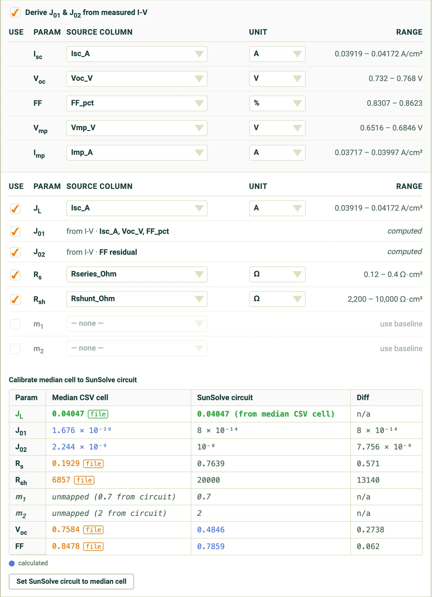
Note that it is recommended to load rather than from measured IV data files. The reason is that the values are often rounded off to a low number of decimal places.
- Click Set SunSolve circuit to median cell.
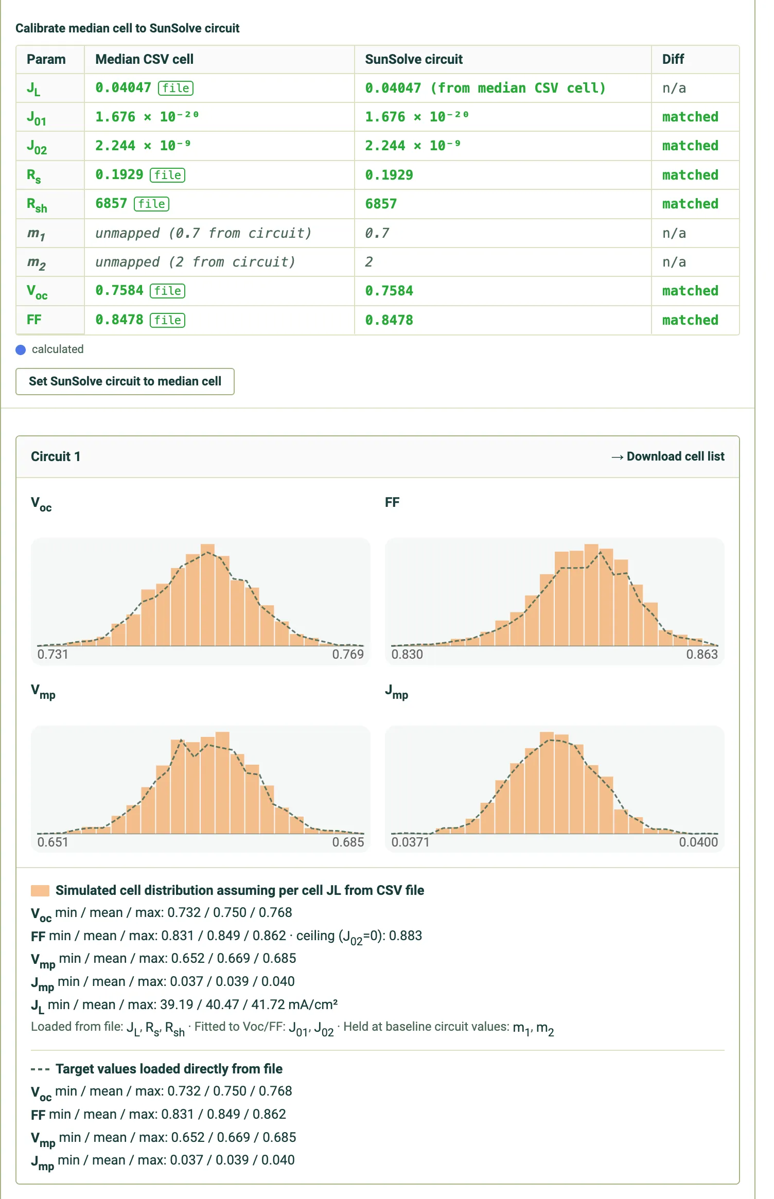
That last step will change the values of , , and in the base circuit within the SunSolve simulation. It will set them to perfectly match the median cell from the loaded distribution. In effect this is fitting the electrical cell model to the measured data. Note that in some cases the baseline electrical model may already be set to acceptable values in which case step 10 can be omitted.
The alignment between the model and the measured cell data can be verified in the table and in the histograms. The dashed line shows the values of and that were loaded from the file. The histogram shows the output of the electrical model, assuming the same as was loaded directly from the cells. That last point is important: the histogram allows the user to check how well the fitting process has replicated the loaded cell distribution.
If the electrical model is well calibrated then the histogram and the target should match. The table also provides an indication of this. In this example there is a good match.
- Click Import.
This will complete the loading process of the cell data.
5. Review the electrical distribution in cell performance
Section link: 5. Review the electrical distribution in cell performanceThe plotted histogram of and for the Modelled cell distribution will now update to reflect the exact values that will be used in the distribution simulation. Initially it may be difficult to spot any difference. The values of the original cell and from the CSV file are shown in dashed orange. Any differences between this orange line and the modelled cells (i.e. the histogram presented in the columns) are effectively cell-to-module losses and gains.
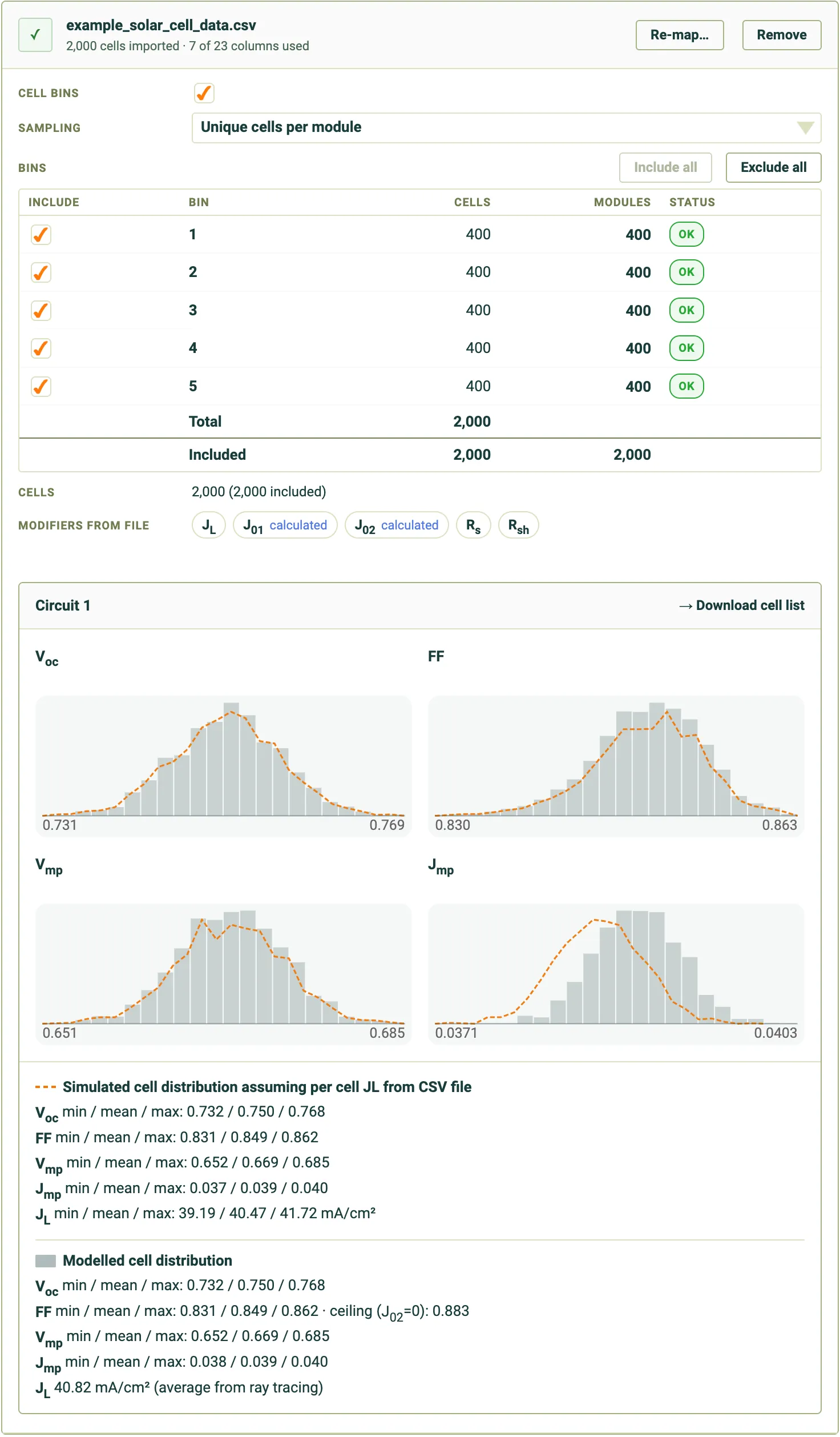
The cell and are now calculated with:
- The SunSolve ray tracing result (the average in the module),
- The SunSolve baseline circuit model (i.e. the values of , , etc.),
- The loaded distribution in cell performance from the file (stored in the simulation as per-cell modifiers).
Point 1 provides a conversion from the CSV loaded cell values that were measured under air, into the module values after encapsulation. The accuracy of that conversion can be improved with well-calibrated baseline models. In this example the small change in is not enough to significantly impact or .
Point 2 provides a means to now adjust the electrical model from describing just a solar cell, into a cell encapsulated within a module. If that conversion included increased edge recombination then that can be added in.
Point 3 carries the distribution in cell performance into the module generation. For example, the distribution in per-cell , which may have occurred due to variations in front-side metal finger width, will now be applied to any distribution in coming from the optical model.
6. Adjust electrical circuit to account for module integration
Section link: 6. Adjust electrical circuit to account for module integrationIt is now possible to update the module electrical inputs to reflect any known changes to the circuit that occur during module fabrication. This may include effects such as edge recombination due to cutting cells and extra series resistance due to the interconnection ribbon. The actual impact these processes may have on an equivalent circuit is highly specific to both the cells and the manufacturing process used. The values may be determined from well-targeted experiments, scientific literature or simulations in more highly detailed electrical solvers.
For this example we will assume that the process to cut the cells in half increases and that the interconnection of cells increases .
- Go to the Inputs > Cell tab.
- Set to .
- Set to .
- Return to the Inputs > Modifiers tab.
The imported per-cell modifiers remain unchanged, so changing the baseline circuit shifts the modelled cell population while preserving its relative distribution. Now the Modelled cell distribution has been updated to reflect the changes to the base circuit. Note that is now lower on average; however, the general shape of the distribution remains. is also very slightly lower. Although this is hard to see on the histogram, it can be read from the values in the text below the graph.
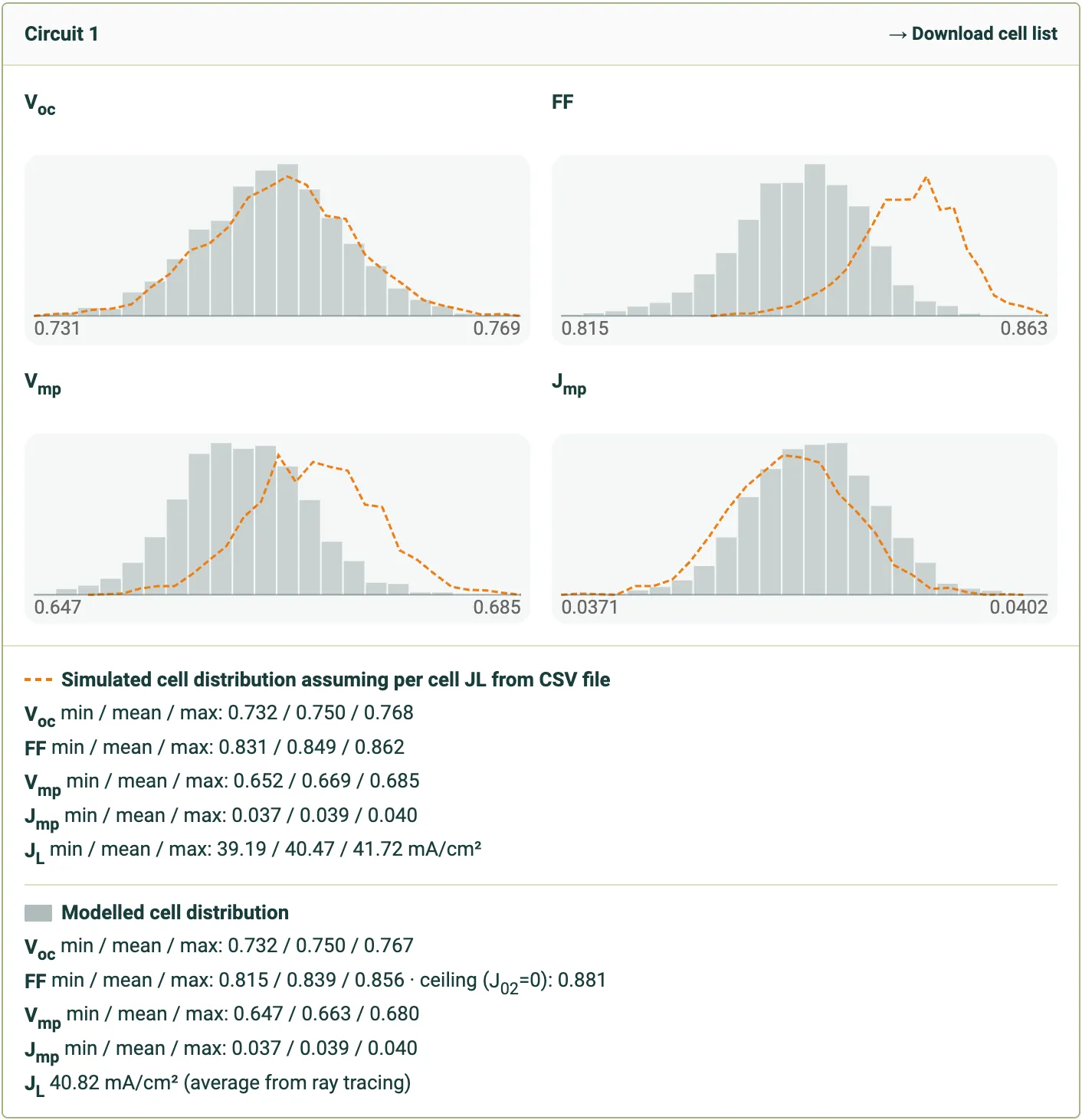
Note that certain circuit inputs are subject to the distributions loaded from the CSV file (e.g. , , , ). Adding a recombination path not subject to distributions is possible via the other components (e.g. the diode).
7. Solve module distribution
Section link: 7. Solve module distribution- Go to the Outputs > Distribution tab.
- Wait while the distribution solves. The output charts will update while the distribution solver is running.
- While the solver runs, the round button at the top left of the tab shows a stop symbol and the summary beside it reads “N samples · sampling…”. Once all 2,000 modules have been solved, the button changes to a green play symbol and the summary reads “2000 samples”. It is now possible to view the results.
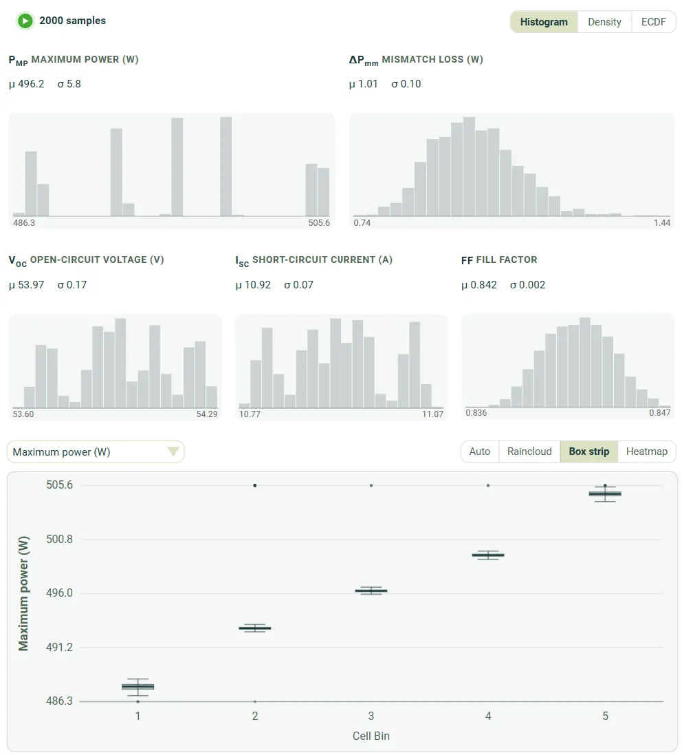
This cell distribution has five distinct cell bins, separated by cell power. This has resulted in five distinct clusters in module output power. The box plot at the bottom of the screenshot shows the module output power versus cell bin. Hover the mouse over any particular cell bin to view where the modules occurred within the histograms.
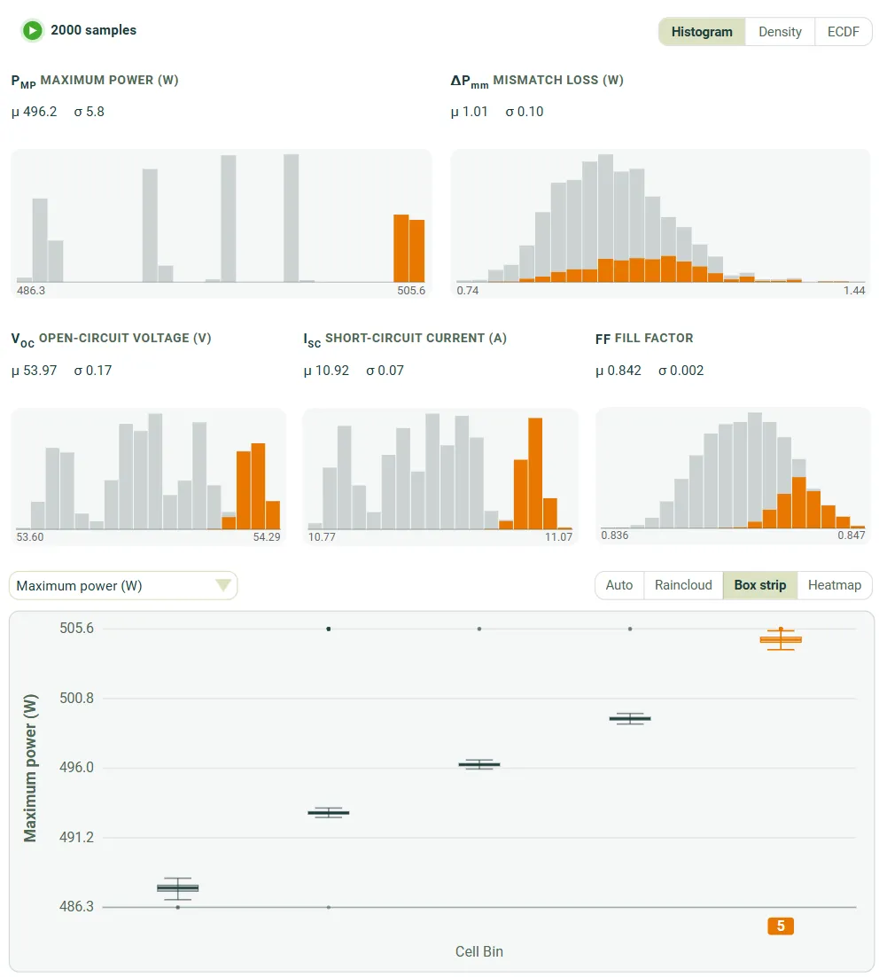
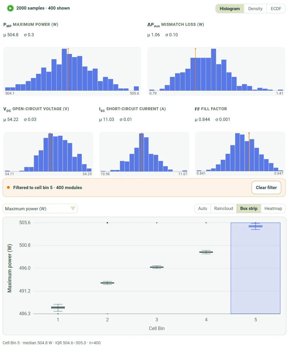
You can also click on the cell bin within the box plot and it will filter the modules in the histograms to match that bin. In the screenshot below the top bin has been selected and now a distribution of modules from the best cell bin is displayed in all of the histograms and in the table at the bottom of the screen.
- Return to the Inputs > Modifiers tab.
- In the Cell bins section, untick the checkbox beside Cell bins.
- Return to the Outputs > Distribution tab. Wait for the solver to run again. It should start automatically.
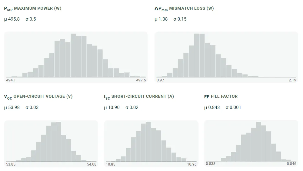
With the binning disabled the modules will be generated with cells selected randomly from all cells. This means that each module will have a mix of cells from all five bins.
The result is a single distribution of module power. The maximum and minimum values are not as extreme as the case shown above with the binning enabled.
Impact of cell location and stochastic noise on mismatch loss
Section link: Impact of cell location and stochastic noise on mismatch lossThere are two additional sources of cell-to-cell variation in that occur in a SunSolve module simulation. It is important to understand how those impact the results. Both of these effects are added to each module in the distribution in an identical fashion.
The first is an artefact of the ray tracing. SunSolve’s ray-tracer uses a stochastic process. If the number of rays per run is low, this can introduce non-uniformity amongst the cells. This distribution is visible on the Outputs > Cell JV tab.
To demonstrate this effect:
- Make a copy of the simulation.
- Go to the Inputs > Options tab.
- Set Rays per run = 5e5 rays.
- Press the triangular run button at the top of the screen to run the optical solver.
- Go to the Inputs > Modifiers tab.
- Check the distribution is loaded and disable the binning.
- Go to the Outputs > Distribution tab.
- Wait while the distribution solves again.
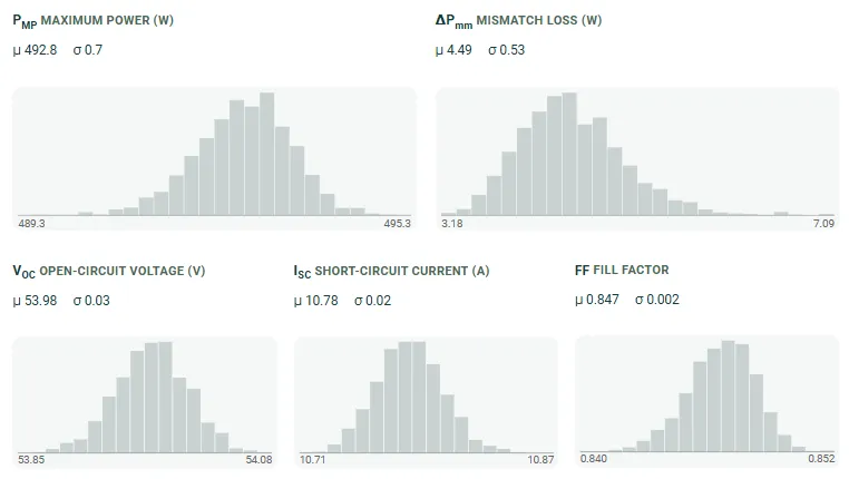
Note that the mismatch loss per module is now much higher. This is the added mismatch due to stochastic noise.
- Go to the Outputs > Cell JV tab. From here you can view how much variation is added to each module.
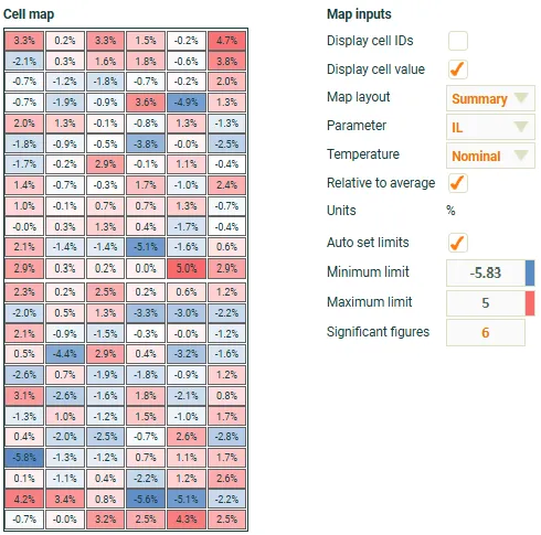
The image below shows the same module, run with 1e8 rays (an extremely high number). It is not recommended to run this as part of the tutorial as it will consume a large number of rays from your account. Note that most of the cells are blue, with certain rows highlighted in red. This is a real optical effect caused by the additional reflective white space at the top, middle and bottom of this layout.
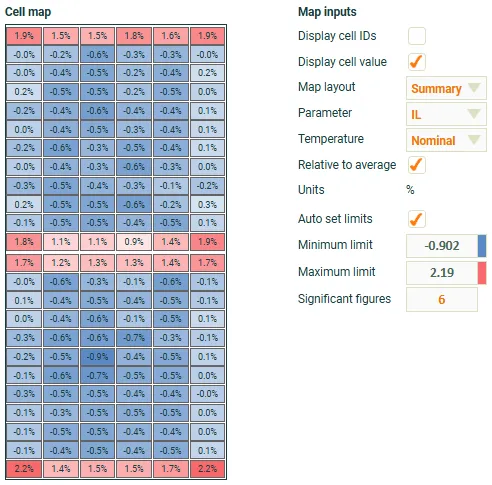
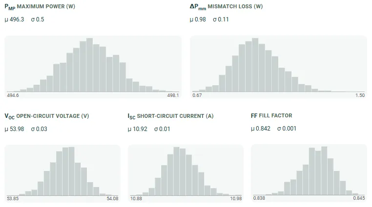
With this number of rays the mismatch loss is reduced, but some amount remains. This residual loss relates to those cells in the hot rows.
We have not shown it here, but a spatially non-uniform light source is another possible cause of a distribution in cell . That effect can be simulated in SunSolve by creating a complex illumination definition based on a measured light distribution from the lab.
Removing the impact of cell location and stochastic noise
Section link: Removing the impact of cell location and stochastic noiseIt is possible to modify the underlying optical model to remove the effects described in the previous section.
- Make a copy of the simulation.
- Go to the Inputs > Options tab.
- Set Device configuration to Unit-cell module.
- Press the triangular run button at the top of the screen to run the optical solver.
- Go to the Inputs > Modifiers tab.
- Check the distribution is loaded and enable the binning.
- Go to the Outputs > Distribution tab.
- Wait while the distribution solves again.
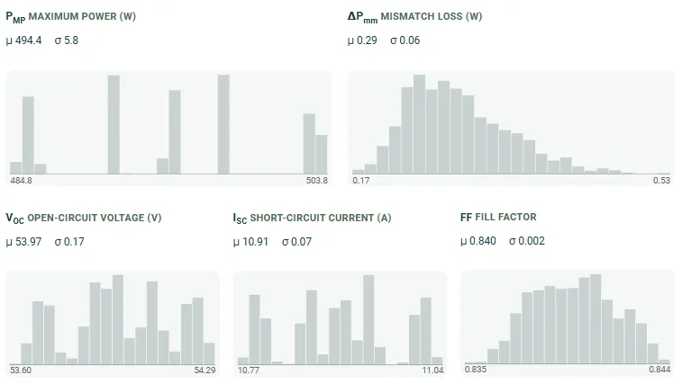
The module distributions now contain no additional variation due to stochastic noise or cell location within the module. This is the purest simulation of the mismatch caused by the incoming cells themselves; however, it lacks the effect of cell position, which tends to be a significant factor.
Related topics
Section link: Related topics- Module population (measured cells) - Reference for the CSV panel
- Module mismatch and cell variation - What each distribution represents
- Distribution results - Interpreting the output
- Simulation options - Device configuration and ray count
Footnotes
Section link: Footnotes-
Half-cut (2x), triple-cut (3x) and quarter-cut (4x) are all in use at the time of writing. ↩