
Module population from measured cells
With the modifiers scope set to Module population and the Distribution source set to Measured cells (CSV), SunSolve Power builds many modules whose cells are drawn from a file of measured cell parameters that you import. This lets you reproduce the module-power and mismatch-loss distribution implied by a real set of measured cells, rather than an assumed statistical distribution.
CSV mode supports a single circuit only. See the modifiers overview for how to enable the feature.
Loading a file
Section link: Loading a fileUse Choose file… to select a CSV, or Paste from Excel to paste tab-separated rows directly. Once loaded, the header reports how many cells and columns were detected. The file stays in a staging state, marked “not yet imported”, until you map its columns and import it.
How file values are applied
Section link: How file values are appliedEach imported cell is expressed relative to the file’s median cell, ranked by Isc. A cell with 2% more J01 than the median cell gets 2% more J01 than the SunSolve circuit, so the measured cell-to-cell variation is applied on top of the simulated module, including its ray-traced optics. Parameters you do not map keep the SunSolve circuit value.
Because every cell is scaled about the median cell, the SunSolve circuit should describe that median cell. The calibration step below lines the two up.
Mapping columns to parameters
Section link: Mapping columns to parametersThe mapping grid has one row per equivalent-circuit parameter. For each parameter you want to take from the file:
- Tick its checkbox to include it.
- Choose the source column from the file.
- Choose the unit the column is expressed in.
- The range of values in that column is shown alongside.
An Isc column must be mapped before importing, because the median cell is chosen by Isc. Parameters left unticked keep the SunSolve circuit value. Columns that are not mapped to any parameter are discarded on import. A ticked parameter needs a source column: Import stays disabled until you choose one or untick the parameter. Check each unit yourself, because the panel does not judge whether a column’s unit looks right.
Deriving J01 and J02 from measured I-V
Section link: Deriving J01 and J02 from measured I-VMeasured data often reports terminal I-V summary values rather than diode parameters.
Enable Derive J01 & J02 from measured I-V to compute the diode saturation currents from measured columns instead of mapping them directly.
Select the Isc, Voc and FF columns and their units; J01 and J02 are then computed for each cell and shown as derived rows in the mapping grid. The Vmp and Imp columns are optional. They are assigned automatically when a column name matches (for example Vmp_V and Imp_A), and can be set to none. Check the unit of each detected column, because it is inferred from the column name and may not match the data.
If J02 is not active in the base circuit, the derive title says so, and J01 is fitted on its own.
Calibrating the median cell to SunSolve
Section link: Calibrating the median cell to SunSolveBefore import, the panel compares the file’s median cell with the SunSolve circuit. The table lists J01, J02, Rs, Rsh, m1 and m2 for both, followed by the Voc and FF each set of values produces, and the difference between them. The circuit is evaluated at the median cell’s photocurrent, so JL never contributes to the differences. A parameter with no mapped column is marked as unmapped and uses the circuit value. Parameters whose branch is not active in the base circuit are left out of the table.
Click Set SunSolve circuit to median cell to copy the median cell’s values into the SunSolve circuit. If Voc or FF still differs from the measured value afterwards, the panel says by how much; review m1 and m2. If the measured FF is at or above the highest FF the circuit can reach, J02 is held at zero and the panel reports it. Parameters whose branch is not active in the base circuit are not changed by this action.
Binning
Section link: BinningReal cells are usually sorted into performance bins before assembly. Binning preserves that structure so that each simulated module is built from a realistic mix of cells rather than a fully random draw.
- Tick Enable binning and choose the Binning by column (for example a bin or grade column) to group the cells. The number of bins and their counts are shown.
- After import, the checkbox beside Cell bins (Use cell bins to construct modules) builds each module from the cells of a single bin.
- The bin table shows a status for each bin: ok, excluded, short or needs resample. Untick a bin to exclude it yourself. Hover over a short or needs resample status to see why — see why a bin is excluded.
The Modules total is shared between bins in proportion to how many cells each bin holds, so a bin with twice the cells builds twice the modules.
Why a bin is excluded
Section link: Why a bin is excludedA bin is left out of the simulation, and none of its cells appear in the results, in two situations. The bin table marks both, and hovering over the status explains which applies.
needs resample, Sampling is Unique and the bin holds fewer cells than one module; switch Sampling to Resample to include it
short, The bin’s share of the included cells is too small to earn a module under either sampling mode
Under Unique, any bin with fewer cells than one module is excluded. Unique never repeats a cell within a module, so a small bin cannot fill one.
Under both Unique and Resample, a bin is also excluded if its cells divided by the total cells of the included bins is less than 1 divided by the number of modules to simulate. The Modules total is shared out in proportion to cell counts, so a bin below that share would be given less than one module.
Because the share is measured against the included bins only, excluding other bins can bring a small bin back in. As a worked example, take a module of 144 cells, Modules set to 500, and three bins holding 100,000 cells in total: LARGE with 99,810 cells, MEDIUM with 150 cells and SMALL with 40 cells. The share cut-off is 1 in 500 (0.2%), which is 200 cells of 100,000.
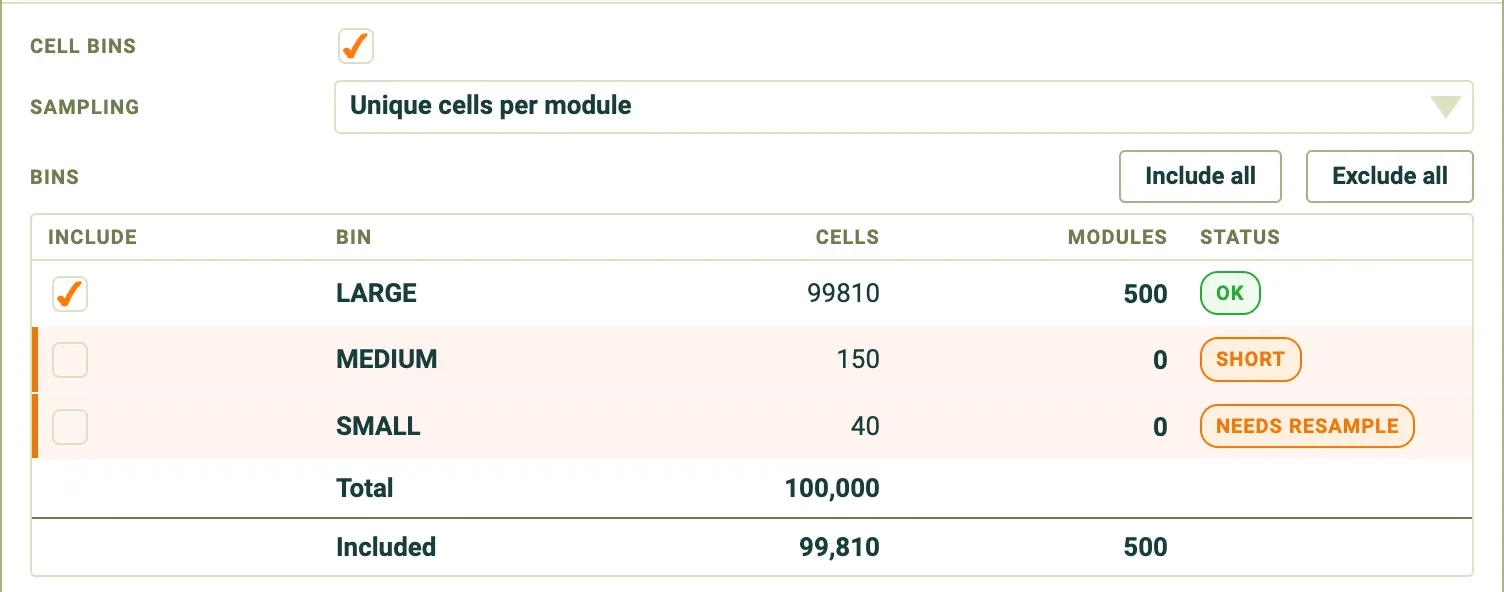
- SMALL has 40 cells, which cannot fill a 144-cell module, so Unique marks it needs resample.
- MEDIUM has 150 cells, enough to fill a module, so Unique does not exclude it for size. Its share is 0.15%, which is below the 0.2% cut-off, so it is short under both modes.
- Under Resample, SMALL is also short, because 40 cells is 0.04%, below the cut-off.
- To include MEDIUM, raise Modules to 700 or more, or untick LARGE. To include SMALL under Resample, raise Modules to 2,500 or more, or untick LARGE. With LARGE excluded, the two small bins share the included cells, so both earn modules. SMALL stays needs resample under Unique.
The tooltip on a short bin gives these numbers for your own bins.
Choosing how cells are sampled
Section link: Choosing how cells are sampledThe Sampling control decides how each module’s cells are drawn from the file, or from its bin when binning is on. Think of the file as a deck of cards, with each module a hand dealt from it.
How cells are drawn, Dealt from the deck: every cell is dealt once before any is dealt again; when the deck runs out it is reshuffled, Drawn and put back: every draw is from the whole file
Across modules, Every cell appears in the same number of modules (give or take one), Some cells appear in many modules and others in none
Bin or file smaller than one module, Bin excluded; with binning off an error is shown, Included; its cells are repeated to fill the module
Best for, Seeing exactly how a known set of cells performs, Estimating the spread of a larger production that the file samples
With a large file, holding a hundred or more modules’ worth of cells, the two options give almost the same results. The choice matters most for small files.
Unique cells per module (default)
Section link: Unique cells per module (default)Each module is filled by dealing cells in turn from a shuffled copy of the file or bin, so no cell appears twice in the same module. The cells’ positions within each module are also shuffled, so the same cell lands in a different place in each module.
Up to the point where the cells run out, this is how a production line would use a batch: set Modules to the number of cells divided by the number of cells per module and every cell is used exactly once. Unlike a production line, the batch is never used up. Ask for more modules than it can fill and the cells are reshuffled and dealt again, so each cell appears in several modules, always in new combinations and never twice in one module.
How often each cell is used depends on the Modules total. For a module of 144 cells:
Things to keep in mind:
- Short bins are excluded. A bin with fewer cells than one module cannot fill a module without repeating a cell, so it is excluded and marked needs resample in the bin table. Its cells still appear in the committed-cell preview and CSV; exclusion only affects which cells are assigned to modules. Whether a bin is too small depends on the number of cells in the module, so changing the module layout can change which bins are excluded. A bin can also be excluded for having too small a share of the cells — see why a bin is excluded.
- Running past the batch narrows the spread. Once cells are dealt again, modules are new combinations drawn from a limited set of cells, so the spread of module power is narrower than a production line built from cells like these would show. The smaller the file, the narrower the spread. This happens whenever the Modules total needs more cells than the file or bin holds.
- Stopping short of the batch leaves cells out. When the Modules total needs fewer cells than the file holds, some cells are not used.
- Excluding every bin still shows all cells. When every bin is excluded or short, the preview and CSV still list every committed cell, but no modules are built.
- Measured Target columns are pre-commit only. Target Voc, FF, Jsc, Vmp, Jmp and Imp appear in the staging preview and download before import, and are blank after import.
- The file must hold at least one module of cells. With binning off, a file holding fewer cells than one module shows a validation error and no modules are built. Choose Resample instead.
Studying cell placement
Section link: Studying cell placementA file holding exactly one module of cells is a useful special case. Every module contains the same cells, so the spread of module power and mismatch loss comes entirely from where each cell is placed: which string or bypass-diode substring it joins, and how much light reaches its position. This measures how much placement matters for a given set of cells, for example to judge whether sorting cells before layup is worthwhile.
What placement can affect depends on the device configuration on the Inputs → Options tab:
Module, Electrical position and position-dependent light such as the extra light near the module edge and cell gaps
With a full module, each position also carries a fixed amount of ray-tracing noise, which is indistinguishable from a real position effect. Raise the ray count until the mismatch loss converges before reading a placement study — see module mismatch and cell variation.
Resample
Section link: ResampleEach position in each module is drawn independently from the file or bin, with replacement, so a cell can appear more than once in the same module and some cells may not appear at all. This treats the file as a sample of a larger population of cells and estimates what modules built from that population would look like, which is a statistical technique known as bootstrapping.
Choose this when the file is a representative sample — for example a few hundred cells measured from a much larger production run — and you want to estimate the spread of modules built from that run, or when you need more modules than the file can supply without reusing cells.
Things to keep in mind:
- Short bins are included. A bin with fewer cells than one module is filled by resampling instead of being marked needs resample. The fewer cells a bin holds, the more often each one repeats: a 20-cell bin filling a 144-cell module uses each cell about seven times, so that bin’s results are dominated by a handful of measured cells. A bin with too small a share of the cells is still excluded — see why a bin is excluded.
- Measured cells are diluted. Even a bin with plenty of cells is sampled with replacement. A bin of exactly 144 cells filling a 144-cell module places only about 91 different cells in each module, with the rest repeated, so some measured cells are left out of each module even though the bin could have filled it exactly.
- Results include sampling noise. Because every module is an independent random draw, the tails of the module-power distribution depend on the seed and on how many cells were measured. A small file gives noisier tails than a large one.
Measured cell area
Section link: Measured cell areaSome mappings need the measured cell area to convert a measured current into a current density. The Measured cell area field shows whether the current mapping requires it; when it does, import stays disabled until an area greater than zero is entered. If the area entered differs from the simulation’s cell area, the panel warns that the difference will scale Isc.
Rows that cannot be used
Section link: Rows that cannot be usedEvery row is checked when the file is staged, before any simulation runs. A row can have one of two problems:
- Failed diode fit: the values are numbers, but no J01 and J02 reproduce the measured Voc and FF. For example, a Voc of 0.
- Invalid input: a value is blank or is not a number, in a column you mapped or in the Isc, Voc or FF column used for the derivation. This includes a blank in a parameter such as Rsh that you only want to adjust.
A row with both problems counts as an invalid input.
If you keep a row with a problem, the values it is missing are taken from the baseline circuit, and the row’s other values are still used. A failed diode fit takes J01 and J02 from the baseline circuit. An invalid input takes the value that could not be read from the baseline circuit. A kept row with a Voc of 0 or below still plots that value in the measured Voc curve, where it shows as an outlier. A blank or non-numeric Voc is not plotted.
When a file has problem rows, a highlighted block just above Import says how many rows have problems, for example “44 of 200 rows have problems”. It has one checkbox for each kind of problem:
- Include N cells with failed diode fits is ticked by default for a new import, so these cells appear in the charts and in the median cell comparison.
- Include N cells with invalid inputs is unticked by default.
Unticking a box removes those cells from the charts, the median cell comparison and the simulation.
A file with no problem rows shows nothing. The counts are exact before you import.
Importing
Section link: ImportingWhen the mapping is ready, click Import. Before importing, the staging note shows how many circuit parameters will receive modifiers. After import you can:
- Re-map… to return to the staging view and change the mapping. This needs the CSV still loaded in the current session; after reopening a document, load the CSV again.
- Remove to discard the imported file.
If the module has more than one circuit, import is blocked with a note that CSV mode supports a single circuit only; remove the extra circuits to proceed.
Frozen at import
Section link: Frozen at importImporting freezes the modifiers and a snapshot of the circuit’s base values in the document, so the simulation keeps using the import you approved. Editing the circuit afterwards does not change them.
Switching off a branch that a committed modifier targets, or moving the breakdown model away from soft breakdown, does not stop the solve and does not change the saved modifiers. The modifiers stay frozen as imported, but whether they have any effect depends on the circuit’s current settings: while the branch is off, or the breakdown model is not soft breakdown, the modifiers for that element have no effect on the result. Switch the setting back and they apply again.
Setting the population size
Section link: Setting the population sizeThe Modules field on the toolbar sets how many modules are built from the imported cells. With Unique cells per module sampling, this also decides how often each cell is used — see choosing how cells are sampled.
Reading the results
Section link: Reading the resultsRun the simulation, then open the distribution results output page to read the module-power and mismatch-loss distributions and download the per-module population. When binning is active, the cell-bin chips on that page let you include or exclude individual bins.
For a worked end-to-end example, including the effect of the device configuration, see how to model module mismatch from measured cells.