Module optics

There are two types of optical models that are used for modules. The first is the ‘simple’ model in which the module active region is treated as a uniform block of cells with look-up tables used to define the surface optics. The second is the ‘complex’ model in which the 3D optical properties can be defined in detail.

See this video for more details on the differences: Module types overview

Assumptions

The following assumptions about the module optics apply to both models:

• There is no spatial variation of any material.

• All solar cells within the module are identical.

• The contacts that connect the tabs (at the top and bottom of the module) do not affect the optical behaviour of the module.

• The optical properties are independent of temperature.

• There is no soiling on the modules during ray tracing (it is applied later during JL solving).

Simple module optics

The simple module uses a simplified optical model for the active region¹ which is optionally combined with a definition of the module frame. The model for the active region neglects many of the 2D spatial variation within the module (e.g. white spaces at the edges and through the centre region of half-cut panels).

Surface

The surface of the active region is modelled via a lookup table which defines, as a function of the angle between the beam and the module, the fraction of incident light that is:

1. reflected (R),
2. lost to parasitic absorption (A_lost) and,
3. absorbed usefully to contribute to light generated current (A_gain).

There are four options to define the surface optics of the active regions in simple modules:

1. Calculate RAT(θ) from materials: an optical material with thin film coatings represents the first interface with air. A lookup table is created using 500 nm light to solve the reflection and absorption as a function of a list of θ values (0, 10, 20, 30, 40, 45, 50, 55, 60, 65, 70, 75, 80, 85, 88, 89). Absorption in thin film coatings is treated as lost and contributes to A_lost. Any other light not reflected is treated as useful and contributes to A_gain. Additional scattering distributions can be defined for the reflected light (see Section 5.5 for a description of scattering models)

2. Interpolate RAT(θ) from table: values of R, A_lost and A_gain are directly entered by user in a table versus incident angle.

3. Interpolate RAT(λ) from table: values of R, A_lost and A_gain are treated as having a wavelength dependence, but no angular dependence. A single definition of this wavelength dependence is entered by the user. This can include a fixed value (i.e. independent of both wavelength and incident angle).

4. Interpolate IAM(θ) from table: a simplified version of option 2 in which no light is reflected and the user defines a table that defines A_gain versus incident angle. This is the model used in view factor analysis and is the set of values that is commonly defined within a pan file.

The lookup table for R, A_lost, A_gain is normalised and defined at a set of discrete incident angles. Linear interpolation is used during ray tracing to determine the exact values to use for any given ray angle.

Scaling of current

Simple modules apply a wavelength‑dependent scalar (short‑circuit current scaling factor) to convert the ray‑traced spectral absorption pattern into module current using a defined QE curve.

See the detailed methodology: Module current scaling in simple optical models

Complex module optics

In the case of complex modules, the complete structure of the modules is defined, and the optics solved in all layers and interfaces as described in the Fundamental optics.

The definition of the modules includes frames, brackets, encapsulant materials (glass, glass ARC, EVA, backsheets), metal tabbing, edge spacing, cell spacing and solar cells. The solar cell definition contains metal electrodes (shape, material, layout), surface textures (e.g. upright random pyramid textures), thin surface coatings (SiNx, SiO2, a-Si, SiOxNy, AlOx etc) and absorber thickness.

Module Frame and Bracket

Module frames can be added to both simple and complex modules. The frame is applied around the outside of the active area.

Frame and bracket geometry

The frame is defined by its width, height, and lip (overhang) dimensions, while the bracket represents the mounting structure beneath or behind the module edge. Together, they form an L-shaped cross-section around the module, as shown in the figure.

• Frame dimensions:

  • Xf / Yf: horizontal thickness of the frame edge
  • Zf: vertical height of the frame (typically 35 mm)
  • Zl: lip height extending over the module glass

• Bracket dimensions:

  • Xb / Yb: horizontal width of the bracket beneath the module
  • Zb: bracket thickness or vertical height

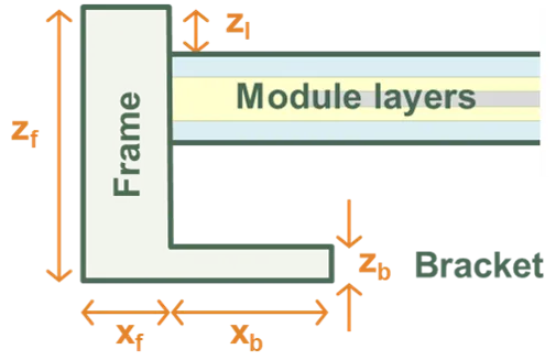Frame and Bracket Definition.

The frame and bracket can be configured as:

• Symmetric: identical on all four sides
• Half-symmetric: identical on two opposing sides (e.g. long edges)
• Asymmetric: fully independent dimensions for each edge

---

Footnotes

1. The active region of the module is the area that includes the cells, glass, EVA, backsheet where absorption of light may result in generation of electrical current. ↩