Stochastic error
Stochastic error is the deviation introduced by tracing a finite number of rays in the Monte Carlo optical solver: fewer rays shorten runtime but increase noise in per‑cell absorption and inflate cell‑to‑cell mismatch; more rays reduce these effects but lengthen solve time and can trigger a >15 min timeout. The goal is to select rays per solar angle that achieve the target module power / mismatch accuracy (e.g. ≤0.1%) without exceeding practical time limits—too few rays randomise the spatial absorption pattern, too many yield diminishing returns and risk failure.
In SunSolve Power the user selects the number of rays to run for each simulation on the Inputs → Options tab using the field Rays per run.
Impact on module output
Section titled “Impact on module output”The magnitude of this stochastic error is demonstrated in the figures below which plot the impact of a varied number of rays on the STC performance of a single panel. In this example the panel contains 144 half-cut cells arranged in two parallel strings with a nominal output power of 440 W at STC. Each ray condition has been run five times.
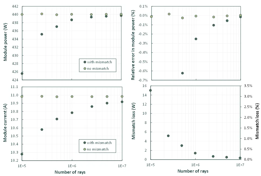 Average STC module power, module current (Isc) and mismatch loss of a 144
half-cell module at STC for various numbers of rays, shown with mismatch (cell connected into module circuit during
solving) and no mismatch (cells solved independently). Error in module power calculated relative to solution with
1x10⁸ rays. Note that the no mismatch case is the average current and the sum of the per cell power. Each point
represents the average of five runs, shown in detail below.
Average STC module power, module current (Isc) and mismatch loss of a 144
half-cell module at STC for various numbers of rays, shown with mismatch (cell connected into module circuit during
solving) and no mismatch (cells solved independently). Error in module power calculated relative to solution with
1x10⁸ rays. Note that the no mismatch case is the average current and the sum of the per cell power. Each point
represents the average of five runs, shown in detail below.
The major impact of running a low number of rays is to introduce a power loss due to cell-to-cell mismatch. When calculated as a sum of cell powers (i.e. when mismatch is neglected) the module power is already within an error of 0.03% for any value of rays run. Once the mismatch is included then it is necessary to run ~2 x 10⁶ rays to reduce that error to 0.1%.
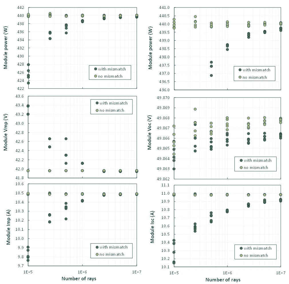 Example 144 half-cell module electrical outputs at STC for various numbers of
rays, shown with mismatch (cell connected into module circuit during solving) and no mismatch (cells solved
independently). Note that the no mismatch case is the average current and the sum of the power and voltage.
Example 144 half-cell module electrical outputs at STC for various numbers of
rays, shown with mismatch (cell connected into module circuit during solving) and no mismatch (cells solved
independently). Note that the no mismatch case is the average current and the sum of the power and voltage.
The next figure plots the distribution in per cell light generated current as a function of the number of rays run. Also shown are the module heat maps for three cases showing the spatial distribution of each cells light generated current relative to the average of the panel. Initially there is a broad distribution in per cell current with a random distribution spatially across the module. For the end case (1 x 10⁸ rays) the distribution is determined by the position of the cells relative to reflective white space (i.e., around the outer edge and through the middle).
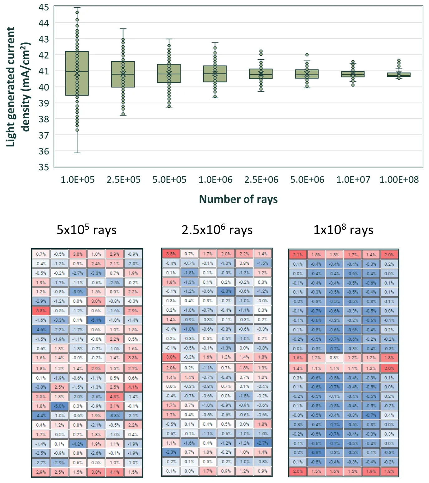 Light generated current in each cell of the 144 half-cell modules shown as a
function of the number of rays run during ray tracing.
Light generated current in each cell of the 144 half-cell modules shown as a
function of the number of rays run during ray tracing.
Some other points worth noting:
-
Crystalline silicon panels contain bypass diodes that limit the overall impact of cell-to-cell mismatch on the output power. If technology with no bypass diodes is simulated (e.g. First Solar CdTe panels) then the impact of running less rays will be more severe.
-
The physical size of the cells will determine how many rays are absorbed. Technologies with larger numbers of very small cell areas (e.g. First Solar CdTe panels) will require more rays.
-
The simulation assumes that all cells are identical. In reality there is likely to be a distribution of cell performance within the module. This distribution will have a similar effect on module output as the stochastic error from the ray tracing.