Illumination

SunSolve Power allows the user to define one or more illumination sources. These sources are used to scale the computed spectral absorbance, reflectance, and transmittance as functions of wavelength into scalar quantities such as equivalent photon current densities. The final result is obtained by integrating over all defined sources.

Note that the choice of spectrum does not determine the wavelength range over which the solution is computed. The wavelength range is configured explicitly on the “Options” tab.

Location

The area of each illumination source can be set to “full area” or “defined”.

A defined-area illumination source can be circular (like in the image below) with a user-defined diameter, or it can be rectangular with a user-defined width and breadth. The local illumination is also assigned a position on the cell (or module), where this position is defined by $x_{\text{offset}}$ and $y_{\text{offset}}$. As shown in the image, these parameters represent the distance from the centre of the cell (or module) to the centre of the local illumination.

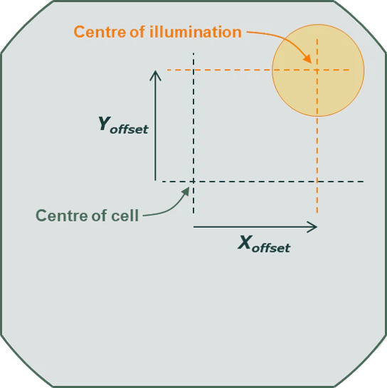
If part of the local illumination does not overlap the cell (or module), that fraction of the illumination will not interract at all with the cell (or module). It will not be attributed to the transmitted fraction of light but to the “remainder”.

Applying local illumination can help ascertain the behaviour of particular regions in a cell or module, such as the fraction of light captured from textured ribbons or from the backsheet between cells.

Angular distribution

There are three options for the angular distribution:

1. Single angle, where the user defines the direction of light by its zenith and azimuth angles. This angular distribution can be considered a delta function.
2. Isotropic, where the zenith angle has a sin θ dependence.* An isotropic distribution is sometimes used to represent diffuse sunlight. It is equivalent to having a uniform radiant intensity (a constant intensity per solid angle).
3. Gaussian, where the zenith angle has an exp[–θ²/(2σ²)] dependence on θ (i.e., a Gaussian function centred at θ = 0). This might represent the illumination from the flat diffuser plate of a cell tester, for which the illumination is meant to be normally incident but actually contains a small angular divergence.

The relative irradiance on a horizontal plane ξ is then given by:

1. ξ = ʃcos θ∙δ(θ)∙dθ / ʃδ(θ)∙dθ = cos Θ, where Θ is the user-defined zenith angle;
2. ξ = ʃcos θ∙sin θ∙dθ / ʃsin θ∙dθ = 1/2;
3. ξ = ʃcos θ∙exp[–θ²/(2σ²)]∙dθ / ʃexp[–θ²/(2σ²)]∙dθ, which approaches 1 for very small σ and 2/π for very large σ;

where the integration limits are θ = 0 and π/2.

Spectrum and incident intensity

The spectral intensity $I_b(\lambda)$ of the selected spectrum is assumed to be the incident intensity of a beam of light on a perpendicular plane. It has the units W/m²/nm. Thus, integrating the spectral intensity over the desired wavelength range gives the beam intensity on a perpendicular plane $\Phi_b$ in W/m².

It is possible to scale this intensity by setting the scaling factor $f$. This value scales $I_b(\lambda)$ equally at all λ.

The irradiance on a horizontal plane is therefore $\Phi_h = \xi \cdot f \cdot \Phi_b$.

We call this prefactor, ξ∙f, the relative horizontal irradiance (RHI). It is calculated and presented as an output for each illumination source.

Here are three examples to explain how measured spectra should be uploaded. In each example, the spectral intensity $I_m(\lambda)$ is measured on a horizontal plane. We recommend that the spectral intensity be first modified to $I_b(\lambda)$ before uploading by multiplying $I_m(\lambda)$ by 1/ξ. Then there is no need to modify the scaling factor $f$.

Example 1. You measure the direct-beam solar spectrum on a horizontal plane when the sun is located at a zenith angle of 30°. Multiply $I_m(\lambda)$ by 1/cos(30°) = 1.154 to give $I_b(\lambda)$ before uploading $I_b(\lambda)$ as a new custom spectrum.

Example 2. You measure the diffuse-sky spectrum on a horizontal plane. This is not uncommon because many measurements of DHI (diffuse horizontal irradiance) are made with horizontally installed pyranometers. If one assumes that the illumination is isotropic (Lambertian), then ξ = 1/2 and you should multiply $I_m(\lambda)$ by 2 to give $I_b(\lambda)$ before uploading $I_b(\lambda)$ as a new custom spectrum.

Example 3. You measure the horizontal irradiance of a cell tester that is known to have a Gaussian angular distribution with σ = 10°. First multiply $I_m(\lambda)$ by 1/ξ = 1.015 to give $I_b(\lambda)$ before uploading $I_b(\lambda)$ as a new custom spectrum.

In all of these examples, we recommend scaling the measured spectrum $I_m(\lambda)$ by 1/ξ to become $I_b(\lambda)$ before uploading. When you do this, you can leave the scaling factor at $f = 1$. The alternative is to upload $I_m(\lambda)$ as the custom spectrum and to set the scaling factor to $f = 1/\xi$. (This will give a relative horizontal irradiance of 1.)

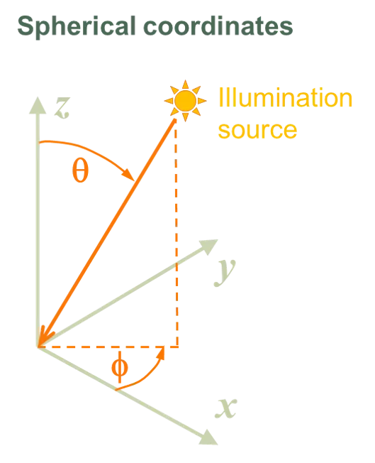
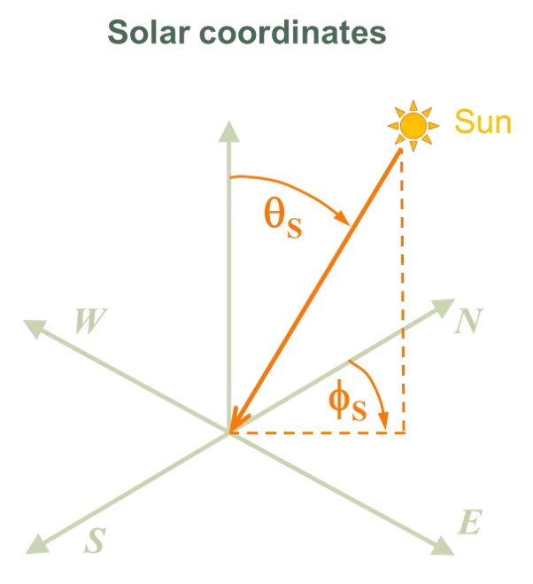
Coordinate system for illumination sources

The coordinate system used to define the location of an illumination source depends on configuration being simulated:

• Spherical coordinates defined from cartesian axes are used when simulating a solar cell or module. In this case, the direction of the illumination source is defined by zenith θ and azimuth φ angles.
• Solar coordinates defined from cardinal axes are used when simulating a system. In this case, the position of the sun is defined by solar zenith $\theta_S$ and solar azimuth $\phi_S$ angles. The relation between the cardinal directions (N, S, E, W) and the xy plane is governed by the inputs entered for the system orientation.

---

*The sin θ dependence arises because the isotropic illumination is treated as having emanated from a hemisphere (like the sky). Thus, the sin θ accounts for there being increasingly more sky as θ increases from directly overhead (θ = 0) to the horizon (θ = π/2). There is no sin θ dependence in the Gaussian distribution because we treat that illumination as having emanated from a horizontal plane (like the diffuse plate of a cell tester).