Optical detector

An optical detector records the fraction of light that leaves the simulated device within a specified range of outgoing angles, rather than over the full hemisphere. You can enable the detector on the Inputs → Options tab by selecting Include detector. Each simulation can include a single detector, but the detector angles that define its acceptance window can be varied using a parameter sweep.

The detector results are reported on the Outputs → RAT and Outputs → Photon currents tabs.

Optical detector angles

The standard results for reflectance and transmittance represent the hemispherical reflectance and transmittance. If the illumination is from the front, then the hemispherical reflectance is the sum of all rays that travel upwards and away from the front of the module, and the hemispherical transmittance is the sum of all rays that travel downwards and away from the rear of the module.

In addition to these standard hemispherical outputs, it is possible to investigate the fraction of rays that travel away from the module within a particular range of angles. This is performed by applying the ‘optical detector’.

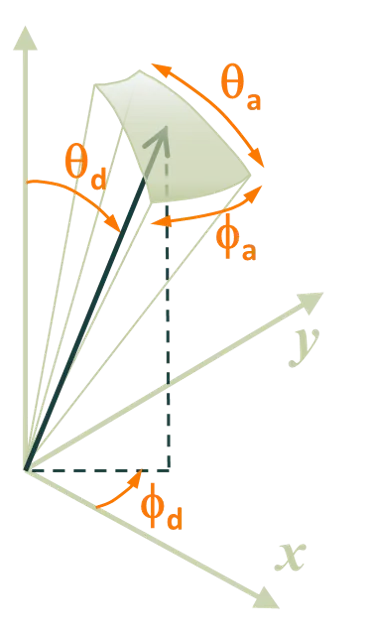
The inputs for the optical detector can be found on the options tab when ‘Include detector’ is checked. These inputs are defined in the figure below. They are the detector and acceptance angles for the zenith ($\theta_d$ and $\theta_a$) and the azimuth ($\phi_d$ and $\phi_a$) of the escaping rays.

The optical detector will therefore detect any ray that travels away from the module at an angle that lies within the bounds $\theta_d \pm \theta_a/2$ and $\phi_d \pm \phi_a/2$.

If ‘limit azimuth angle’ is not checked, then the azimuth angles are assumed to be $\phi_d = 0°$ and $\phi_a = 360°$. In that case, $\phi_d$ is irrelevant because when $\phi_a$ is 360°, the optical detector will detect rays of any φ.

Uses for an optical detector

Researchers often quantify the scattering from a sample by its ‘haze’. The haze is the ratio of scattered to total light for either reflectance or transmittance. It is experimentally determined with a spectrophotometer by combining the results for hemispherical measurements (with integrating sphere) and specular measurements (without integrating sphere).

SunSolve can be used to simulate the haze measurement with inputs that represent a typical spectrophotometer setup. For example, one might set the incident illumination angle to 8°, and the detector zenith angles to $\theta_d = 8°$ and $\theta_a = 10°$, with no limits placed on $\phi_a$.

SunSolve can also be useful to evaluate the reflectance as a function of angle $\theta_d$. For example, one might sweep $\theta_d$ with 9 steps from = 5° to 85° with an acceptance angle of $\theta_a = 10°$, and with no limits place on $\phi_a$.

Warning

The ‘optical detector’ is not located at a single location. It is effectively above (or below) the entire module. It is simply limited to a finite range of ray angles.

When the acceptance angles are small, it is probably that only a small fraction of rays will be detected by the detector. In that case, the random error in the detector results will be much larger than the random error for the hemispherical reflectance or transmisttance.

When evaluating the results as a function of angle, it is often satisfactory to have large acceptance angles, or even to place no limits on $\phi_a$. In that case, the signal from the optical detector will be larger and therefore the random error will be smaller.