Optical scattering

Scattering models

Optical scattering is implemented by one of three models: ‘no scattering’, ‘Lambertian scattering’ or ‘Phong scattering’. These models are represented by the diagrams below.

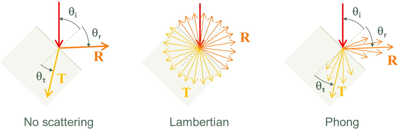
Whenever a ray intersects an interface, SunSolve first determines if the ray is reflected or transmitted using the stochastic approach described on the ‘General’ tab. SunSolve then determines the new direction of the ray, where this direction depends on the scattering model.

With no scattering, the ray’s new direction is determined by assuming that the interface is specular and hence the reflectance angle $\theta_r$ equals the incident angle $\theta_i$ and the transmitted angle $\theta_t$ is given by Snell’s law.

With Lambertian scattering, the spherical-polar angles (θ and φ) that define the ray’s new direction are determined stochastically from

$$\theta = \arccos \left( {\chi^{\frac{1}{2}}} \right),$$

and

$$\phi = 2\pi\chi,$$

where χ is a random number, 0 ≤ χ < 1, and where unique random numbers are generated to determine θ and φ.

With infinitely many rays, these equations lead to Lambertian reflection (or transmission), whereby the light intensity per solid angle is uniform. Notice that the new ray direction is independent of $\theta_i$.

With Phong scattering, SunSolve determines the new direction as

$$\Delta\theta = \arccos\left ({\chi^{\frac{1}{\alpha + 1}}}\right )$$

and

$$\phi = 2\pi\chi,$$

where α is called the Phong exponent, and where Δθ is the difference between the new angle and the specular reflection, Δθ = θ – $\theta_r$, or the specular transmittance, Δθ = θ – $\theta_t$, depending on whether the ray is reflected or transmitted. This follows Schümacher’s implementation of the Phong model for stochastic ray tracing.

Thus, Phong scattering is identical to Lambertian scattering when α = 1 and $\theta_i$ = 0 (normal incidence), and it is identical to ‘no scattering’ when α is infinite—although α = 1,000,000 is high enough to emulate a specular surface. SunSolve limits α to 1 ≤ α ≤ 1,000,000.

The figure below shows how the probability function $f(\Delta\theta) = (\cos\Delta\theta)^{1+\alpha}$ depends on Δθ and α. Note: this is not the intensity function.

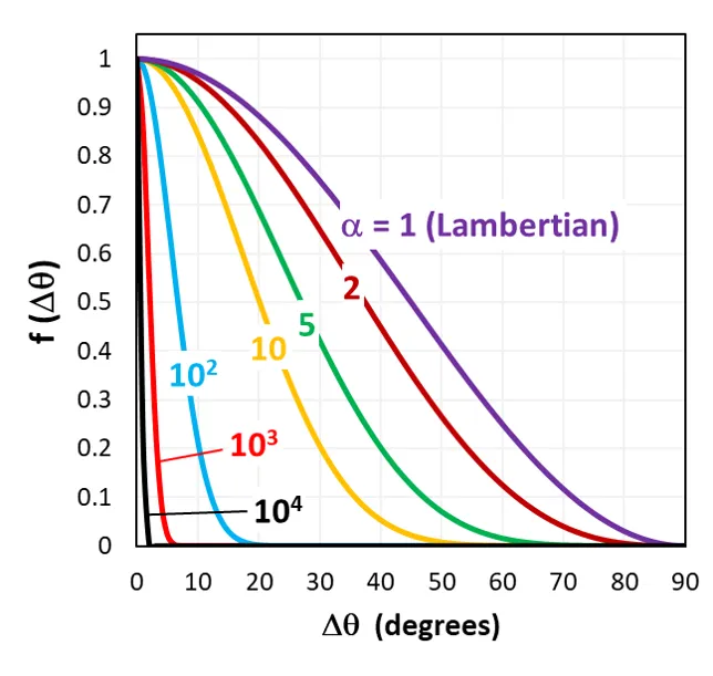
Notice from the above figure that Phong scattering can be used to simulate ‘focused’ scattering. For example, with α = 1000, the scattered light for a reflected ray will be approximately θ = $\theta_r$ ± 5°. This might be useful when simulating random pyramids whose base angles vary by ± 5°.

Scattering fraction

There are two approaches to computing the fraction of incident rays that are scattered.

The first approach is to set a constant scattering fraction Λ. This means that for each ray that interacts with the surface, Λ of these will be scattered by the chosen scattering model and the remainder will not be scattered. Thus, setting Λ = 0 will mean that there is no scattering, no matter what scattering model is selected.

The second approach is to apply the scalar scattering-model. With this model, the scattering fraction Λ is not constant but decreases with increasing wavelength. This fraction also depends on the incident angle, the refractive index of the materials and whether the ray is reflected or absorbed.

For reflection,

$$\Lambda = 1 - \exp\left [- ( \frac{2\pi}{\lambda} \cdot \sigma_{\text{rms}} \cdot 2 \cdot n_i \cdot \cos\theta_i) ^ 2 \right],$$

and for transmission,

$$\Lambda = 1 - \exp\left [- ( \frac{2\pi}{\lambda} \cdot \sigma_{\text{rms}} \cdot \left| n_i \cdot \cos\theta_i - n_t \cdot \cos\theta_t \right | ) ^ 2 \right],$$

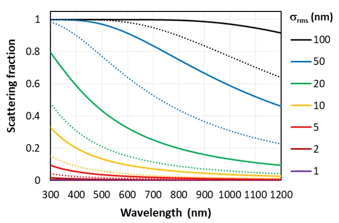
where $\sigma_{\text{rms}}$ is the root mean square roughness of the surface.

The figure below plots the scattering fraction as a function of wavelength and $\sigma_{\text{rms}}$ for an incident medium of $n_i = 1.5$ where the incident angle is either $\theta_i = 0°$ (solid) or 50° (dotted), as determined from the scalar-scattering model.

Additional notes

We make three additional comments.

Firstly, when either Lambertian or Phong scattering is imposed at a surface, SunSolve randomises the polarisation of the ray after it interacts with the surface. In such case, the Phong model might, in fact, yield slightly different results to when there is no scattering and polarisation is tracked.

Secondly, with both Phong scattering and non-normal incidence ($\theta_i > 0$), there’s a possibility that the new ray direction has θ > 90°. If this were allowed, it would mean that a reflected ray is actually transmitted, or a transmitted ray is actually reflected. SunSolve does not allow θ > 90° for the Phong model: whenever the calculated θ > 90°, the direction is recalculated to be θ – 90°.

Finally, we comment on the implementation of the Phong model for stochastic ray tracing, which follows the approach taken by Schümacher and applied elsewhere. (Not all of these papers are explicit about the equations they used but their authors have confirmed to PVL their approach.)

Phong’s seminal equation for scattering was conceived for rendering graphics and not stochastic ray tracing. As a consequence, there is ambiguity in its implementation and we encourage feedback and discussion on this issue.

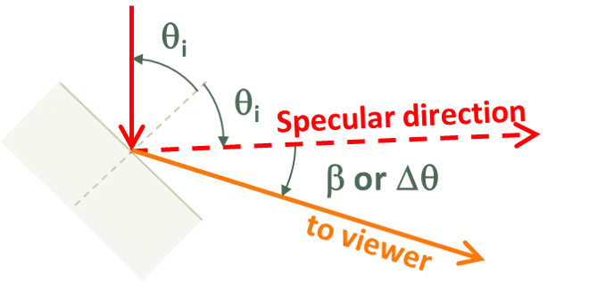
We paraphrase Phong’s definition as this: the relative intensity of light that reflects from a surface to a viewer is $R$ [cos β]^α, where $R$ is the reflectance of the surface and where β is the angle beteen the viewer and the direction of the reflected light if it were specular. (We called this angle Δθ earlier.) Furthermore, both the source and the viewer are infinitely far from the surface.

Hence, after accounting for Lambert’s cosine law, which translates to a cos β reduction in illumination intensity, the fraction of photons reflected by the surface at β must be $R$ [cos β]^{α + 1}.

How should this function be applied to ray tracing? That’s unclear. From an ideal ray-tracing perspective, no rays will be reflected at exactly β and hence the intensity at β should be zero. Instead, we must define the fraction of rays that propagate within some solid angle, such as the infinitessimal solid angle $d\Omega = \sin\theta d\theta d\phi$, from which we can determine the probability that the ray propagates between 0 and β, and thence the probability function $f(β)$.

When this approach is applied to isotropic illumination (e.g., Lambertian reflection) where the reflected intensity per $d\Omega$ is constant, the probability function can be derived as

$$f(\beta) = -2\int_{0}^{\beta}\cos{\theta}\sin{\theta}d\theta = \left(\cos\theta \right)^2.$$

Thus, if we take Phong’s definition of intensity to be that within $d\Omega$, then the probability function would be

$$f(\beta) = -2\int_{0}^{\beta}\left(\cos{\theta}\right)^{\alpha}\sin{\theta}d\theta.$$

If, on the other hand, we take Phong’s definition of $R$ [cos β]^α to be the intensity distribution between 0 and β, then the probability distribution becomes the simple equation:

$$f(\beta) = \left(\cos\beta \right)^{\alpha+1}.$$

The first of these approaches might make more sense in light of Phong’s definition, but the latter is simpler and has been implemented before. In either case, Lambertian scattering is equivalent to α = 1, which is pleasing but not necessary. (It’s possible that other researchers have also implemented f(θ) = [cos β)]^α in which case Lambertian scattering is equivalent to α = 2.)

In conclusion, SunSolve applies Schümacher’s implementation of the Phong model but we welcome discussion on alternatives.