Solver modes

There are three solving modes in SunSolve Power:

1. Single solution,
2. Sweep,
3. Optimisation.

In single-solution mode, the results are calculated using the input values on the many input tabs. A simulation contains a single run.

In sweep mode, the user selects certain inputs to be ‘swept’. These selected inputs are stepped from an initial value to a final value, and the results will be returned as multiple runs under the same simulation. Almost every input—even materials—can be swept.

In optimisation mode, the user selects certain inputs to be optimised and an optimisation goal, where the goal includes an ‘output metric’ and whether that metric should be maximised or minimised. SunSolve then determines the values of the selected inputs that meet the optimisation goal. This requires SunSolve to conduct multiple runs under the same simulation.

Note that SunSolve’s optimiser applies a genetic algorithm that is well suited for complicated optimisations, such as those with more than one input. A simple optimisation with a single input might be more efficiently solved with a sweep.

Optimisation routine and options

We now describe the optimisation routine. The underlined words are user options.

The optimisation solver uses a genetic algorithm to find the optimal input values. This algorithm follows an evolution-based approach to find the ‘fittest’ combination of genes (optimisation inputs) over multiple generations.

The user sets the number of runs per generation $N_G$. Every run is populated with all of the inputs defined on the various input tabs, except those selected as optimisation inputs (genes). The values for the optimisation inputs will be assigned by the optimisation routine.

In the first generation, the number of runs is either $N_G$ or $3^n + 1$, whichever is higher, where $n$ is the number of inputs being optimised. The gene values are selected so that they cover the full range between the user-defined lower and upper bounds for each input. The first generation also includes the user’s best guess.

All runs within the first generation are then solved in parallel, and the output metrics are collated. The runs with the best output metric (i.e., the fittest runs) are added to the ‘gene pool’. As the generations continue, the gene pool will always consist of the fittest runs, where the size of the gene pool cannot exceed runs in gene pool $N_{\text{GP}}$.

A second generation of runs is then created, where the gene values are selected by ‘mating’ the runs from the gene pool. This mating process involves the mix fraction $s$ and the maximum mutation M_max. The mating process is described in more detail below.

At the completion of the second generation (and all subsequent generations), the gene pool is again modified such that it contains the $N_{\text{GP}}$ fittest runs from all generations.

The generations continue until one of the following termination conditions are met:

1. the user stops the simulation by clicking stop ■,
2. the maximum runs is reached,
3. the maximum total rays is reached
4. the time limit is reached,
5. the run failure threshold $f$ is surpassed, or
6. the algorithm converges (defined below).

At that point, the run that gives the maximum output metric is defined as the ‘fittest’. Its gene inputs are loaded for the final run, which is solved to give the optimised results.

Termination conditions

The first four termination conditions are self-explanatory.

The fifth termination condition arises when the number of failed runs in the gene pool exceeds $f$. A failed run occurs when there are failures within the ray tracing or electrical solving routines. If this arises, you’re welcome to send PV Lighthouse the SIM file that caused the problem and we’ll ascertain what went wrong.

The sixth termination condition, convergence, is the most desirable condition. It means that the solver found the optimal inputs (subject to the specified constraints).

The definition of convergence is complicated by the Monte Carlo approach taken by the ray tracer. Since the Monte Carlo approach is stochastic (contains randomness), we would like the uncertainty of the optimal inputs to be small relative to the uncertainty in the stochastic behaviour of a single run.

Specifically, we define convergence as

$$\text{CI}_{\text{GP}} < k \cdot \text{CI}_{\text{BR}},$$

where CI_GP represents the 95% confidence interval of the runs in the gene pool, CI_BR represents the 95% confidence interval of the best run, and $k$ is a user-defined constant called the convergence tolerance.

We demonstrate the meaning of this convergence condition using the graphs below.

These graphs plot the results of two separate cases. Each case constitutes a simple simulation that contains one input variable and a gene pool of just 8 runs, each with a different input value.

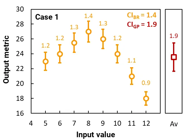
The orange circles plot the output metrics for each run in the gene pool, and the orange error bars (and labels) show their 95% CI. This CI arises from the stochastic nature of the ray tracing. The CI of the best run is CI_BR.

The red squares plot the average of the output metrics, and the red error bars (and label) show the 95% CI of the runs in the gene pool; this CI is CI_GP and it quantifies the variability in the output metric of the gene pool. (The calculation of CI_GP does not depend on the 95% CI of the runs.)

In Case 1, the gene pool contains runs with highly variable output metrics, where CI_GP = 1.9, which is significantly larger than the CI of the best run, CI_BR = 1.4. Thus, if $k$ were set to 1, the simulation will not have converged. Another generation of runs would be populated with input values closer to 8 (the value of the best run) and the solver would continue.

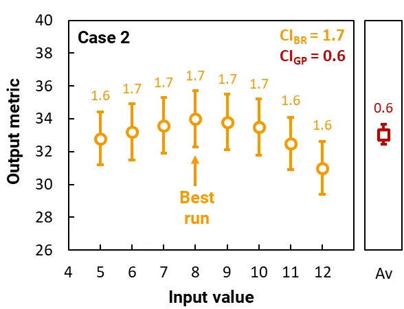
In Case 2, the gene pool contains runs with a similar output metric, where CI_GP = 0.6, which is significantly smaller than the CI of the best run, CI_BR = 1.7. Thus, if $k$ were set to 1, the simulation will have converged. The optimal input would be 8, and the maximum output metric would be 34 ± 1.7.

Mating procedure

The best $N_G$ runs are each mated with another randomly selected member from the gene pool. This creates $N_G$ children whose genes are a mix of their parents’ genes. The value of those genes, i.e., their inputs, are determined by the following approach:

$$X = X_2 + \Delta X \cdot s \pm R \cdot \Delta X \cdot M_{\max},$$

where R is a random number between 0 and 1, X is the input value of interest, and ΔX = X₁ - X₂; and where X₁ and X₂ are the input values of the fitter and poorer of the two parents, respectively.

The image below demonstrates this approach for a two-dimensional optimisation; i.e., when there are two input varaibles, X and Y. It depicts the two parents as grey dots within the X–Y parameter space, where X₁, Y₁ is the fitter and X₂, Y₂ is the poorer of the two parents. The new child will be randomly generated anywhere within the shaded red square of the parameter space.

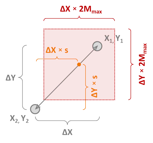
Thus, a larger M_max will lead to a greater variability in the children of the next generation. A larger M_max will also tend towards a more robust but slower optimisation algorithm. The optimal values for s and M_max depend very much on the problem being solved.

Finally, we mention that the algorithm clips the ‘red square’ so that it does not extend beyond the user-defined lower and upper bounds for the inputs.