System configuration

Premium SunSolve accounts are able to simulate modules mounted within a system. You can enable this type of simulation on the Inputs → Layout tab by selecting Configuration: System.

A system is comprised of one or more identical modules. The modules can be tilted relative to the ground and they can be mounted using posts, torque-tubes and clamps. The ray tracing incorporates reflection from the ground and from the various mounting components. The electrical behaviour of each module is determined independently, accounting for cell-to-cell electrical mismatch within each module. The current version of SunSolve does not account for module-to-module mismatch.

Note that SunSolve Power provides limited scope for simulation of systems. Where more detailed system simulation is required it is necessary to use SunSolve Yield.

System image

A 3D rendering of the system to be simulated is displayed at the top of the System inputs page. This image is representative of the simulation inputs and will update itself as you change those values. The unit-system block to be simulated is shown within a wire frame and includes modules coloured to look like realistic devices (note that the module colours, including the backsheet, are not based on simulation inputs). During the optical simulation, any ray that strikes the side walls of the unit-system keeps the same direction and intensity, but has its location translated to the opposite boundary of the unit system. This has the effect of simulating an ‘infinite field’ made up of unit-system blocks. This is represented in the image as ghost modules. The image only shows a finite number of rows and ghost modules, however within the simulation this would extend to infinity. An example image is shown below.

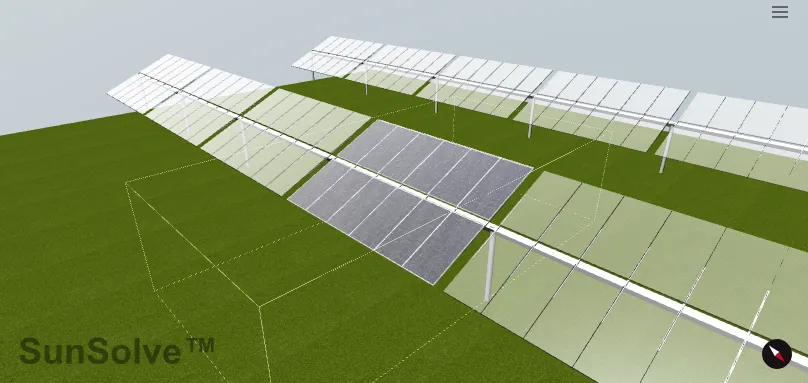
The image can be rotated using your mouse and zoomed in/out with the mouse wheel. It is also possible to shift the image by holding the control key while using the mouse to move the image. In the bottom right corner is a compass with the red arrow pointing north.

You can edit the appearance of the image by clicking on the three lines icon in the top right. This will allow you to hide the unit-system box and to change the appearance of the ground. It is important to note that this has no impact on the simulation, it is just to allow the creation of nice images. That same menu has the option to download a *.png file containing the system image.

If the image is taking too long to render itself, or is otherwise in the way, then you can minimise it by clicking on the ‘System image’ text in the top left. The image will not redraw itself while it is minimised.

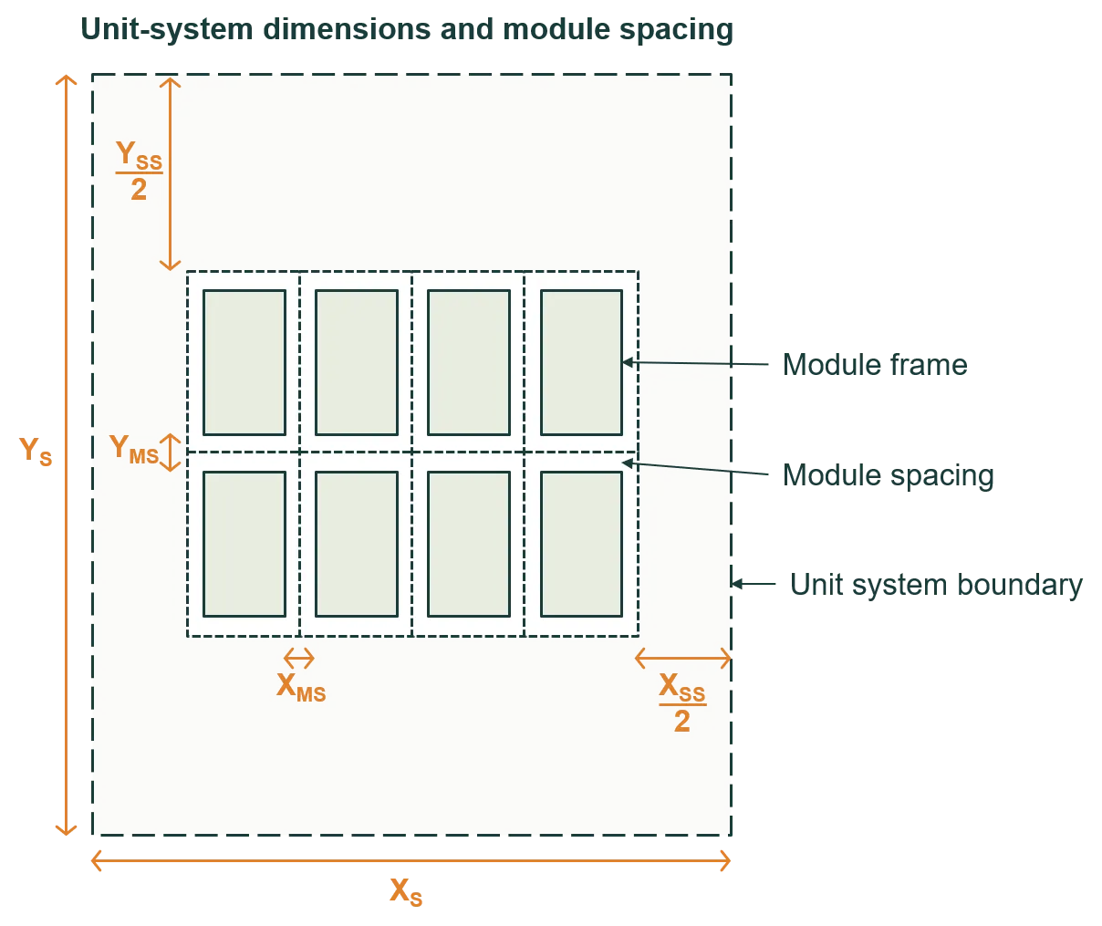
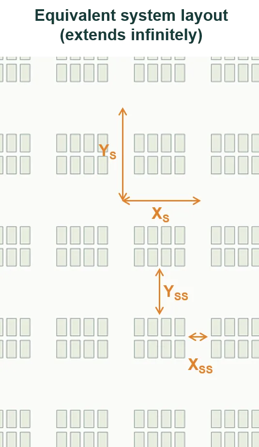
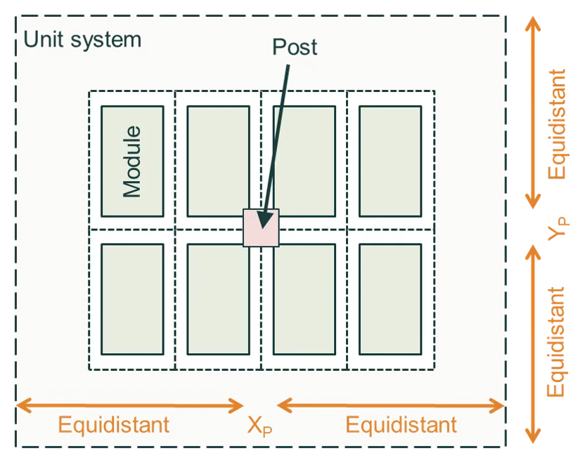
System dimensions

The first figure below defines the dimensions of the ‘unit system’ as well as the spacing between modules $X_{\text{MS}}$ and $Y_{\text{MS}}$. The dimensions $X_{\text{S}}$ and $Y_{\text{S}}$ define the full extent (or pitch) of the unit system, whereas $X_{\text{SS}}$ and $Y_{\text{SS}}$ define the spacing between groups of modules within a unit system. The unit-system spacing is in addition to the module separation.

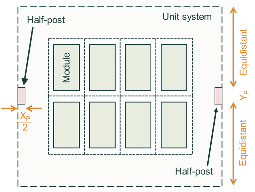
The second figure shows the layout of a system when it’s represented by the unit system of the first figure. The system contains infinitely many unit systems – which in this example contains 2 × 4 modules – and therefore it extends infinitely in both X and Y directions.

When defining the dimensions of the unit-system dimensions, the user has three options: (i) to define the pitch $X_{\text{S}}$ and $Y_{\text{S}}$, (ii) to define the spacing $X_{\text{SS}}$ and $Y_{\text{SS}}$, or (iii) to define the row pitch and the lateral spacing. If the tilt orientation of the modules is in the X direction, the row pitch is equivalent to $X_{\text{S}}$ and the lateral spacing is equivalent to $Y_{\text{SS}}$; whereas if the tilt orientation is in the Y direction, the row pitch is $Y_{\text{S}}$ and the lateral spacing is $X_{\text{SS}}$.

For a large PV system – e.g., a system with hundreds of modules – we’re most interested in the performance of a ‘central module’. A central module is a module that’s sufficiently far from all sides of the system that its unaffected by edge effects. (Edge effects tend to be significant in the first and last row of a system, and in the five modules modules at either end of a row.)

To simulate a central module, simulate a unit system with a single module and zero module spacing, and then set appropriate unit-system dimensions. The figures below show an example unit system (left) and its equivalent system (right), which extends infinitely in X and Y directions.

System components

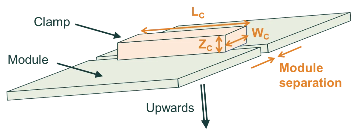
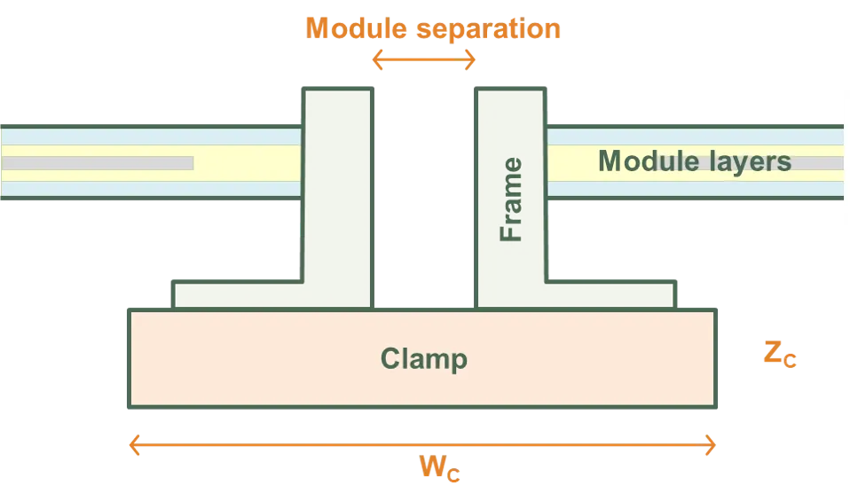
Clamps

SunSolve treats clamps as rectangular prisms. The figures below define their dimensions.

The clamps lie immediately below the module frame (or immediately below the module layers if there is no frame). In the XY plane, the centre of the clamp coincides with the centre of the module separation.

The clamp length must be less than the length of the module; the clamp width must be less than the width of the module plus the module separation; and the clamp height $Z_{\text{C}}$ must be less than whichever is smallest: $Z_{\text{MT}}$, $Z_{\text{MP}}$ or $Z_{\text{MG}}$ (see definitions below).

Clamps do not protrude beyond the module spacing into the space surrounding a module row.

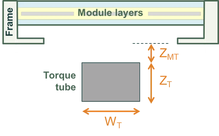
Torque tube

The modules of a single-axis tracking system are mounted on a torque tube, which rotates as the sun passes through the sky. The figure below illustrates a single-axis tracking 1P system with a cylindrical torque tube; ‘1P’ stands for one module in portrait.

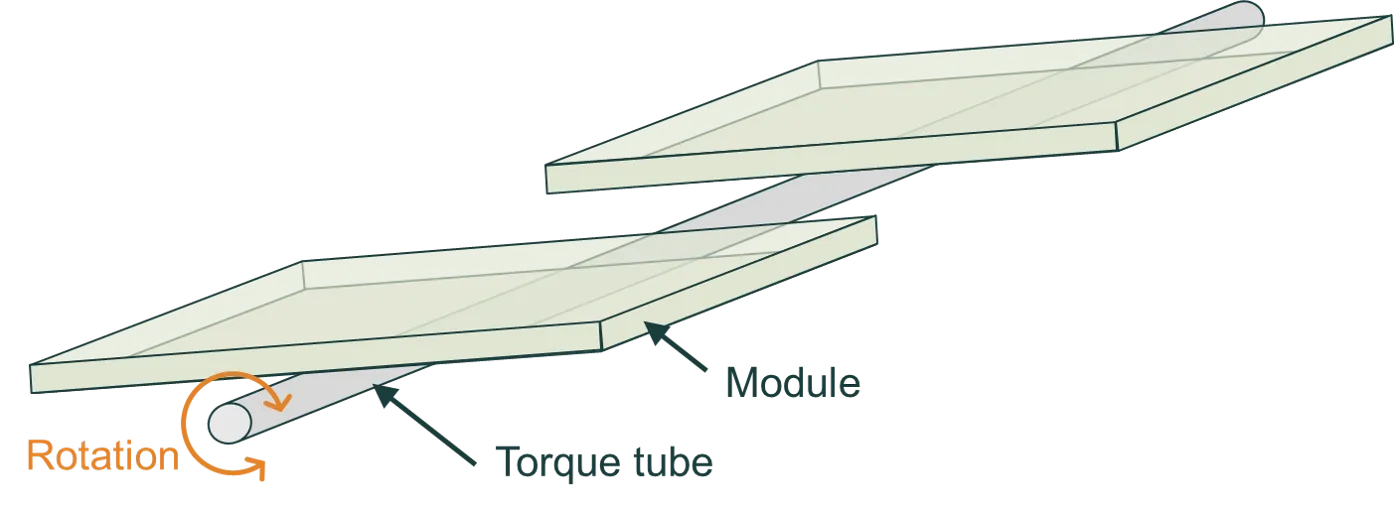
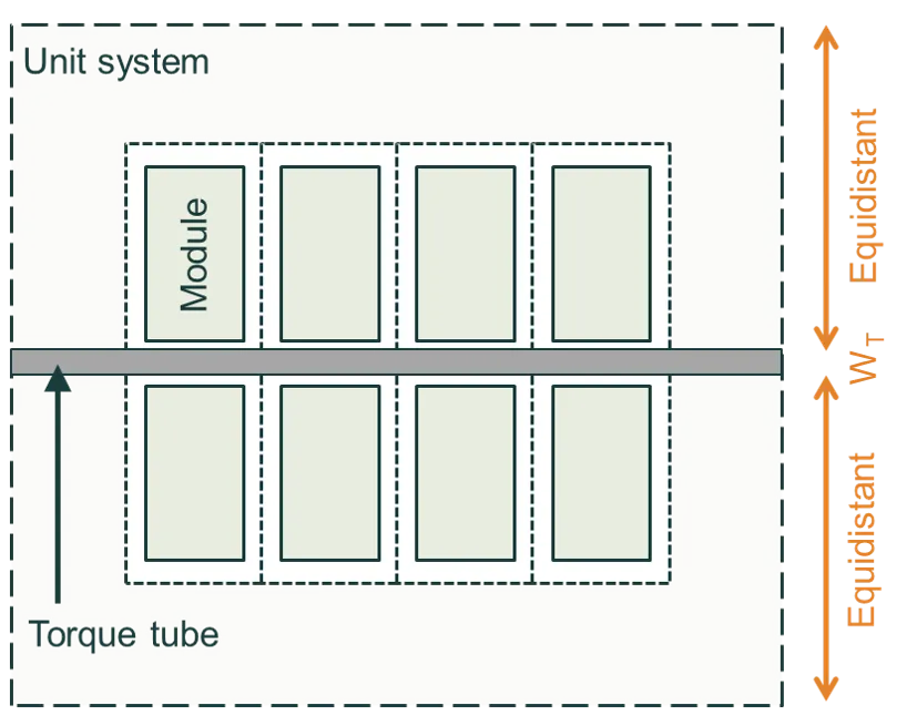
SunSolve can account for the shading and reflectance from both cylindrical and rectangular torque tubes. The figures below define the dimensions. The first figure shows a cross section of a 1P tracking system with a rectangular torque tube. The second figure shows a plan view of a 2P tracking system.

The torque tube is centrally located within the unit system and it extends to the edge of the unit system. If the modules tilt in the Y direction then the torque tube is aligned to the X axis, like in the image below. If the modules tilt in the X direction, the torque tube is aligned to the Y axis.

Posts

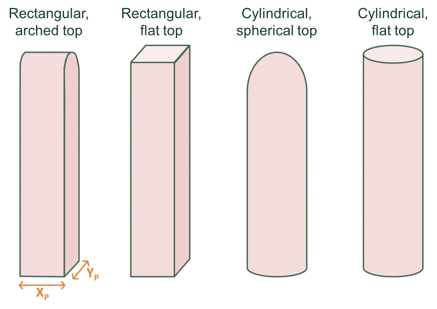
Posts can be rectangular with an arched or flat top, or they can be cylindrical with a spherical or flat top. The figure below illustrates these options.

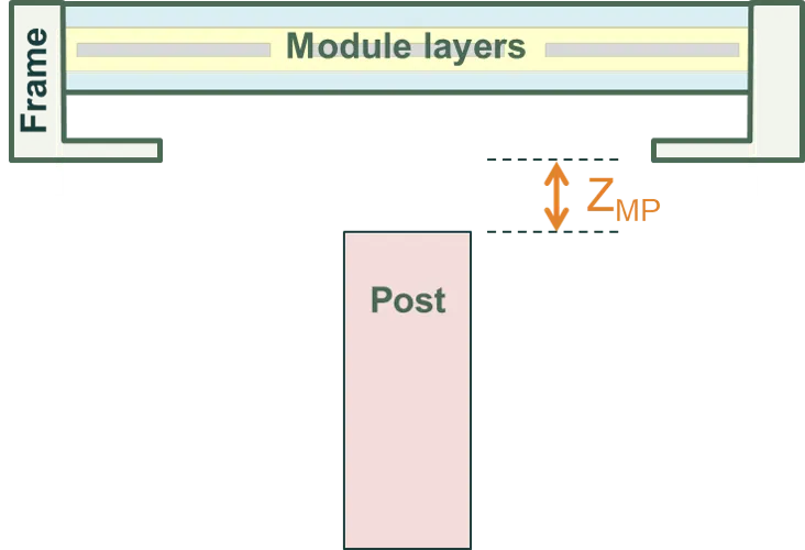
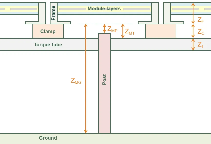
The figure below shows the height of a post is defined by its distance from the bottom of the frame (or from the the bottom of the module layers if there is no frame).

In this version of SunSolve, there are two possible locations for the posts. The options are shown in the figures below: (left) the post is at the centre of the unit-system, and (right) the post is centred on the axis of the torquetube but located at the edge of the unit-system.

System height, tilt and axis of rotation

Height definitions

The figure below defines the vertical distances of the system components.

The most significant distance is $Z_{\text{MG}}$, the height of the bottom of the module (including its frame) above the ground. The height above the ground of the clamps and torque tube, and the height of the posts, are all defined from $Z_{\text{MG}}$.

All of these definitions are specific to a horizontal module; i.e., they assume the module tilt is zero.

Tilt orientation and direction

The modules of a system can be tilted in either X or Y directions. This allows you to tilt them in portrait or landscape, irrespective of how many cells are assigned to the X and Y directions.

The modules are then faced in any direction of the compass, as defined by the modules’ azimuth angle $\phi$ relative to due north.

For example, the figure below first shows how a module is defined in x/y coordinates. This module has two columns in the x direction and four rows in the y direction. The module is then tilted in the y direction by an angle $\beta$ (where a postive $\beta$ makes the front of the module face in the positive y direction). Finally, the module is assigned an orientation $\phi_{\text{M}} = 112.5°$ such that the front of the module faces east–south–east (for a positive $\beta$).

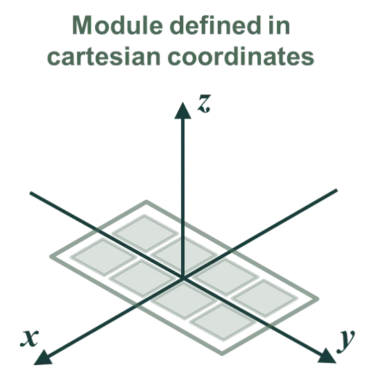
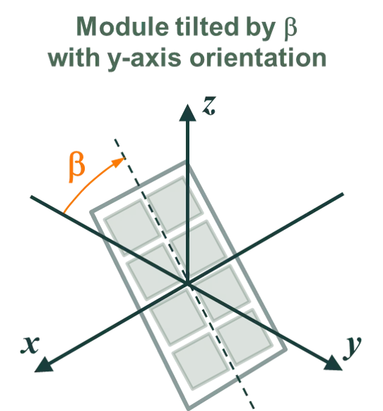
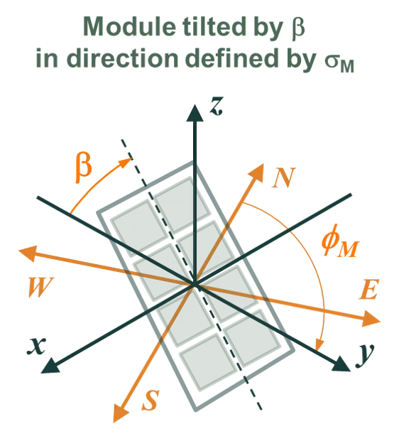
Note that in this example, a negative $\beta$ would make the module face west–north–west.

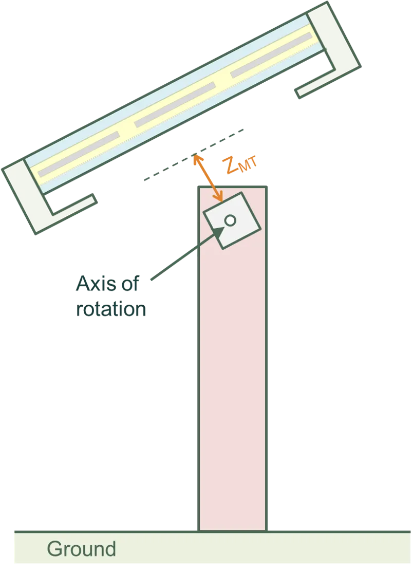
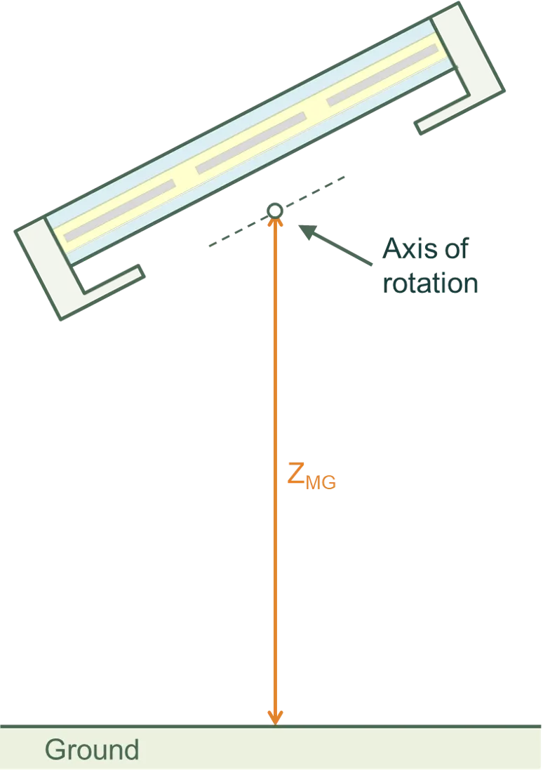
Axis of rotation for tilted modules

The axis of rotation depends on whether a torque tube is included in the simulation.

With a torque tube, a non-zero tilt causes a rotation of the module, clamps, and torque tube about the axis of the torque tube.

Without a torque tube, a non-zero tilt causes a rotation of the module and clamps about the axis passing through the middle of the module in the XY plane and the bottom of the module in the Z plane.

In either case, the posts remain stationary.

The figures below indicate the axis of rotation with and without a torque tube.