Viewing Results
This tutorial continues from the previous quick-start guide, Running Your First Simulation. Before beginning, make sure you have a completed simulation selected (see the previous tutorial for setup steps).
In this tutorial you will learn how to:
- View simulation outputs in SunSolve Yield
- Plot performance metrics (for example, cell-to-cell mismatch loss)
- Request aggregated or hourly data over selected date ranges
- Generate detailed cell heat maps, separated by direct, diffuse, front, and rear absorption
- View and download a Waterfall chart of losses
In this example, results are shown for the DC output of a single module.
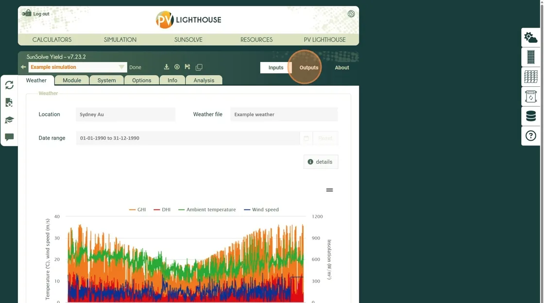
Open the outputs workspace
Section titled “Open the outputs workspace”SunSolve includes several tabs dedicated to viewing the results of a completed simulation. You can explore these for any project that has finished running.
Step 1. Click Outputs to open the output workspace.
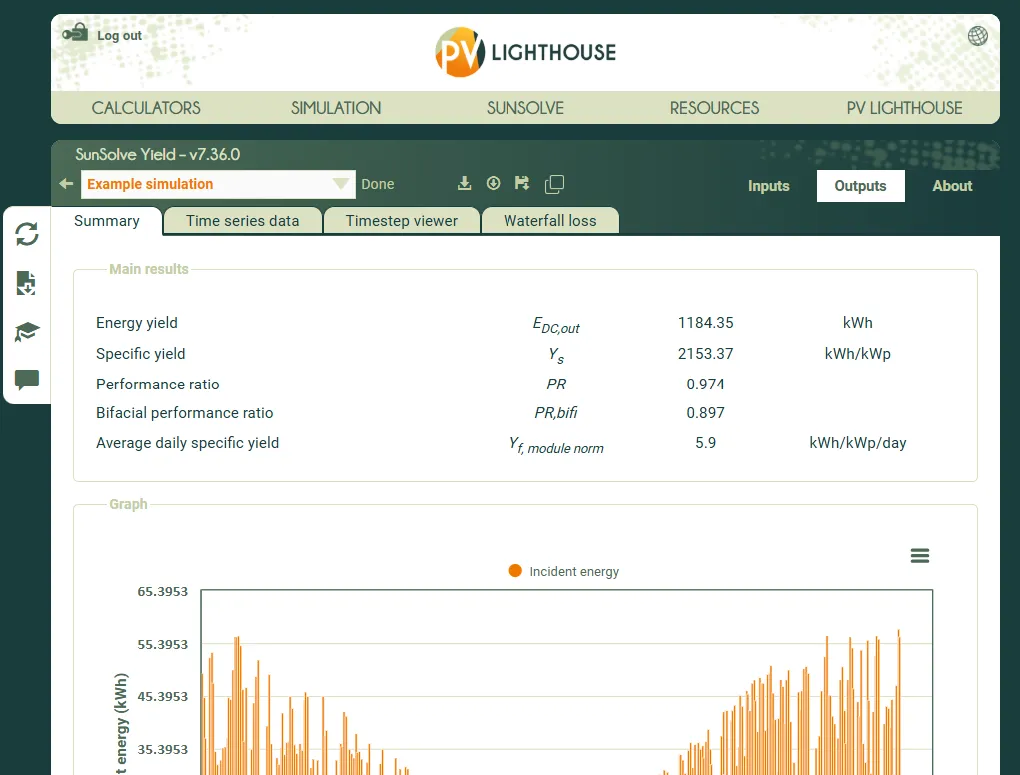
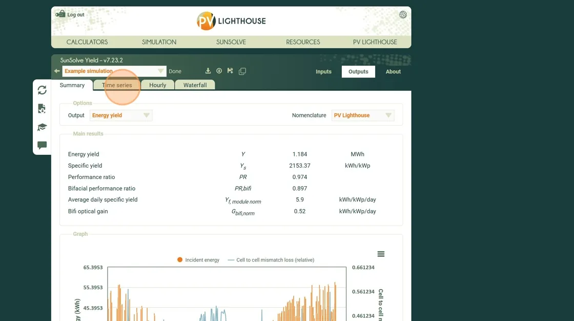
Output yield summary
Section titled “Output yield summary”The Summary tab provides an overview of key outputs that can be plotted as a function of day of year or month.
This allows a quick visual check of the results and helps identify important seasonal or operational trends.
Refer to the Technical Reference Guide for detailed definitions of each output parameter.
As an example, let’s add a plot showing the cell-to-cell electrical mismatch loss over the year.
Step 2. Click Summary to view the integrated results of the simulation.
 Step 3. Scroll down the page to view the chart. From the list of variables, select Cell-to-cell mismatch loss (relative) as the plot option for the Y axis.
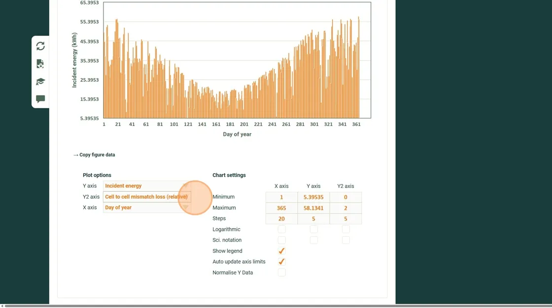
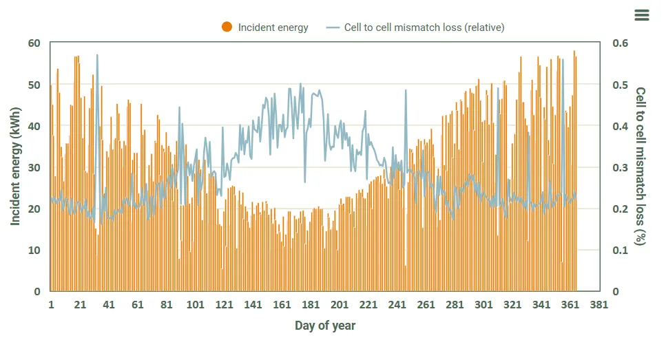
You can explore other output variables and examine how they vary throughout the year. Use this view to check for any unexpected trends or anomalies in the simulation results.
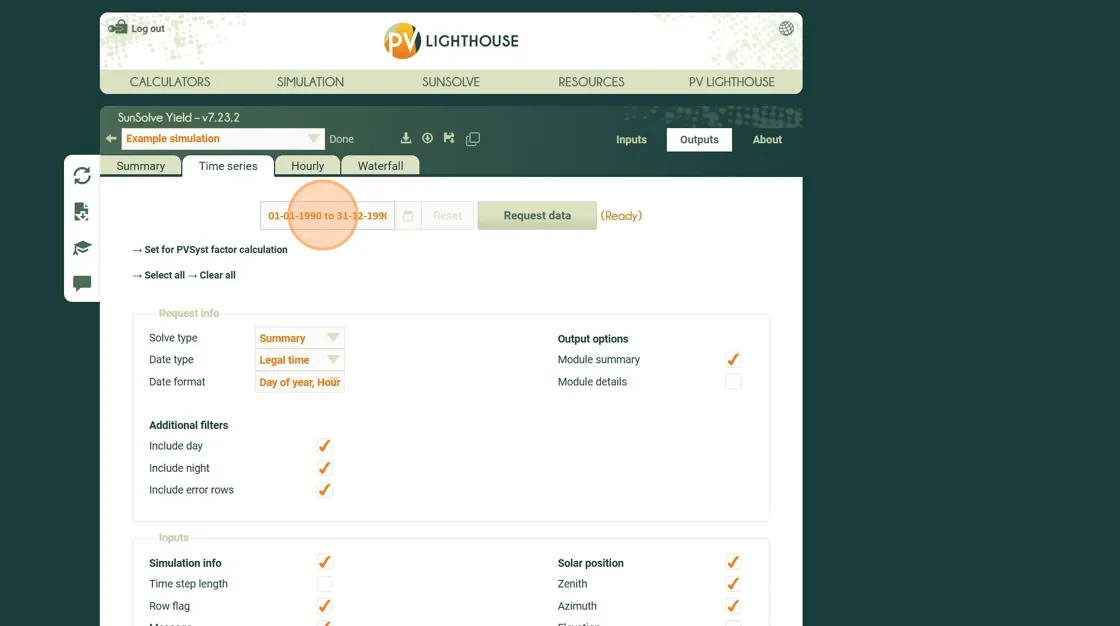
Download hourly time-series data
Section titled “Download hourly time-series data”SunSolve records a large number of data fields at each time step. These can be downloaded into a CSV file for further analysis or use in other software.
The following steps demonstrate how to download a combination of weather inputs and module outputs for a specific date range.
Step 4. Click Time series data to open the time-series output tab.
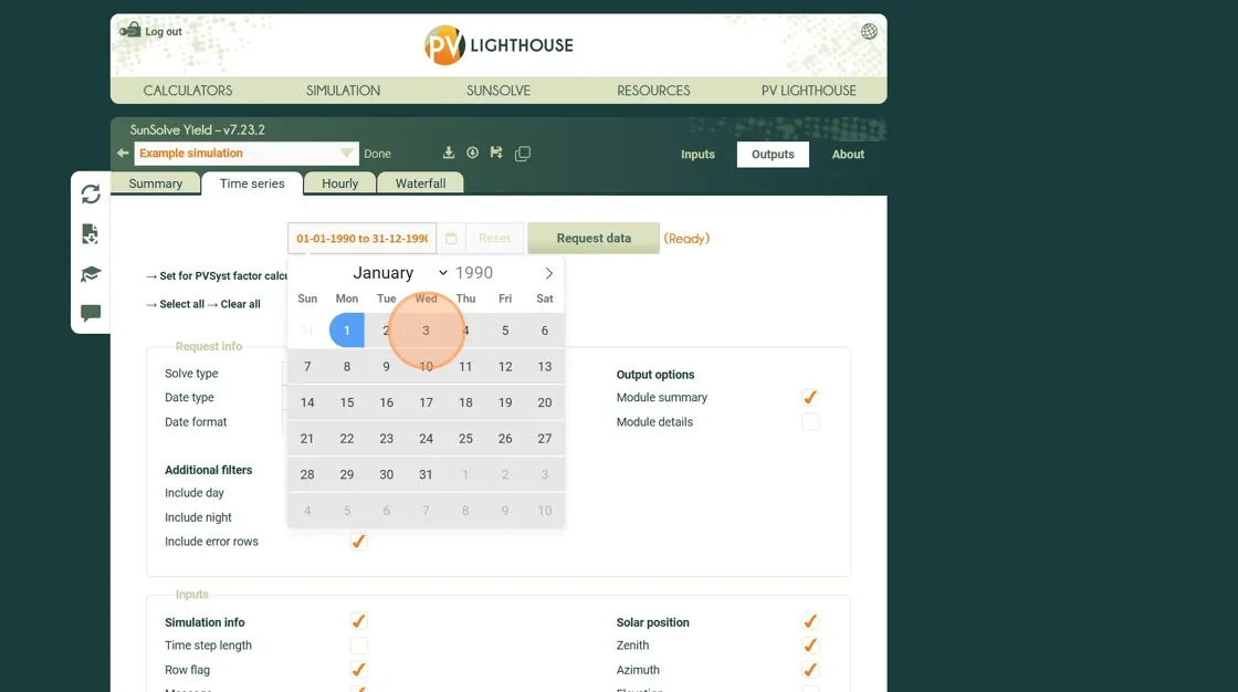
Step 5. Click the Select Date Range field.
Step 6. Select day 3 to set January 3rd as the start date.
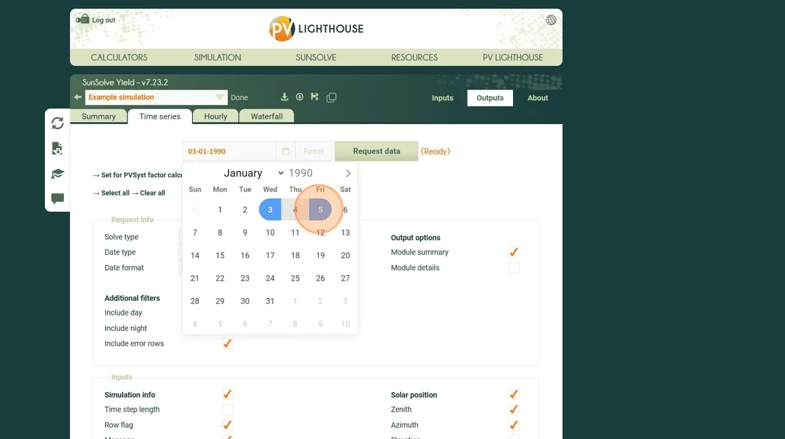
Step 7. Select day 5 to set January 5th as the end date.
Step 8. Under Output options, enable Module summary to include the module-level electrical results.
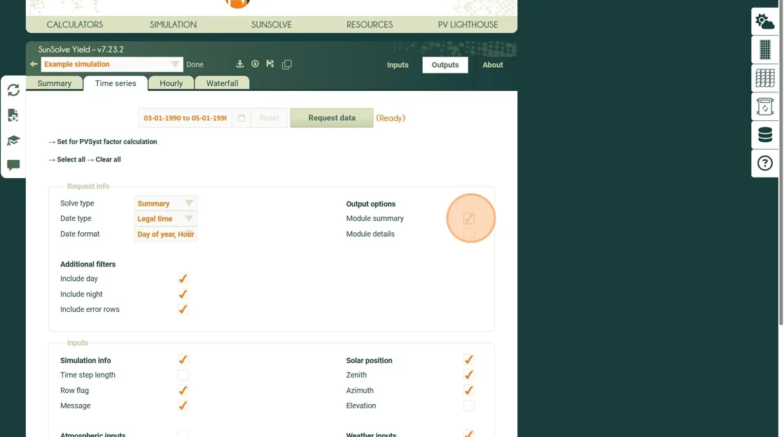
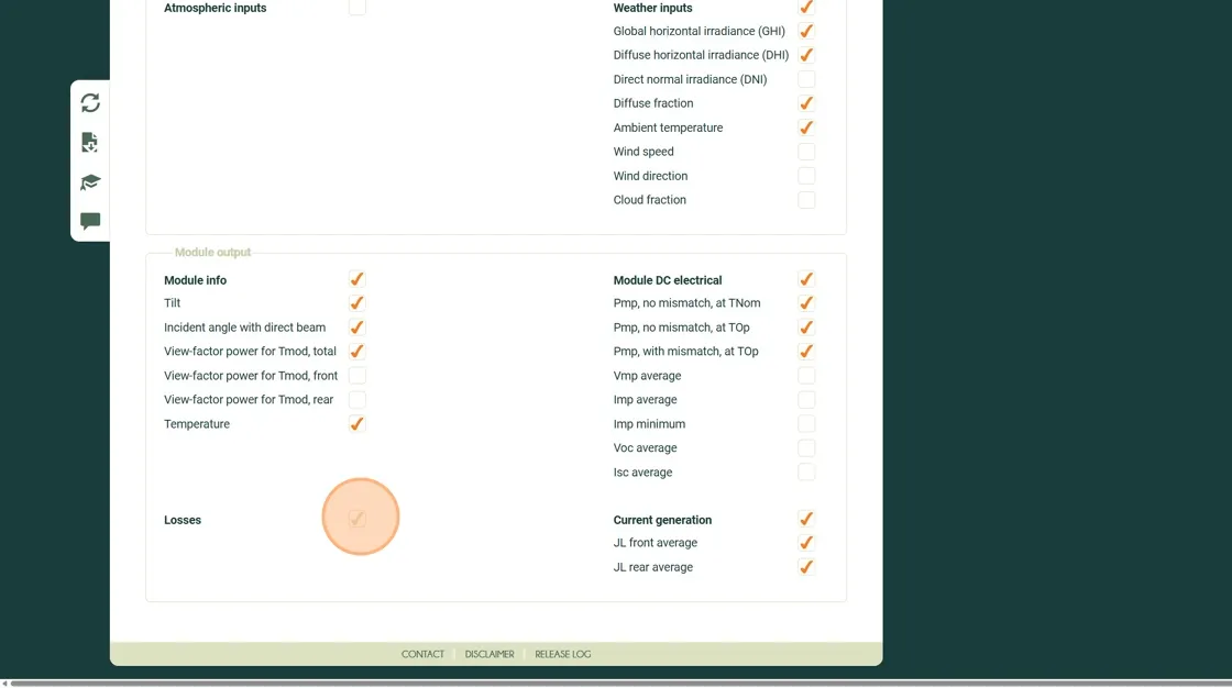
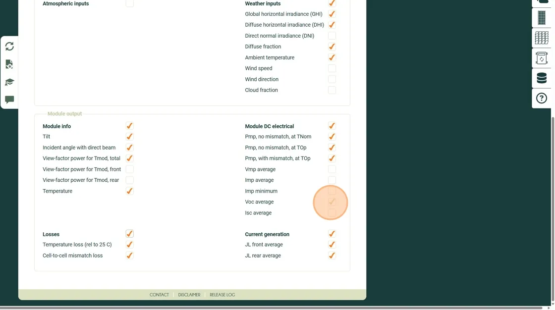
Step 9. Scroll to the bottom of the page and choose the desired module outputs.
In this example, select Losses and Voc average.
 Step 10. Click Request data to begin the download process.
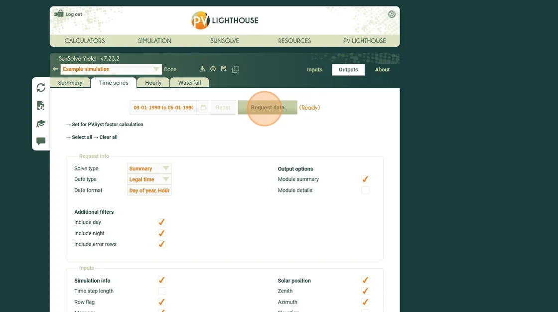 The request is sent to the server, which retrieves the required data.
Progress appears next to the Request data button, and you can cancel the request at any time.
Once complete, the file will automatically download to your local machine.
The request is sent to the server, which retrieves the required data.
Progress appears next to the Request data button, and you can cancel the request at any time.
Once complete, the file will automatically download to your local machine.
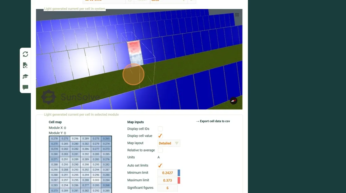
Retrieve hourly data and examine detailed results
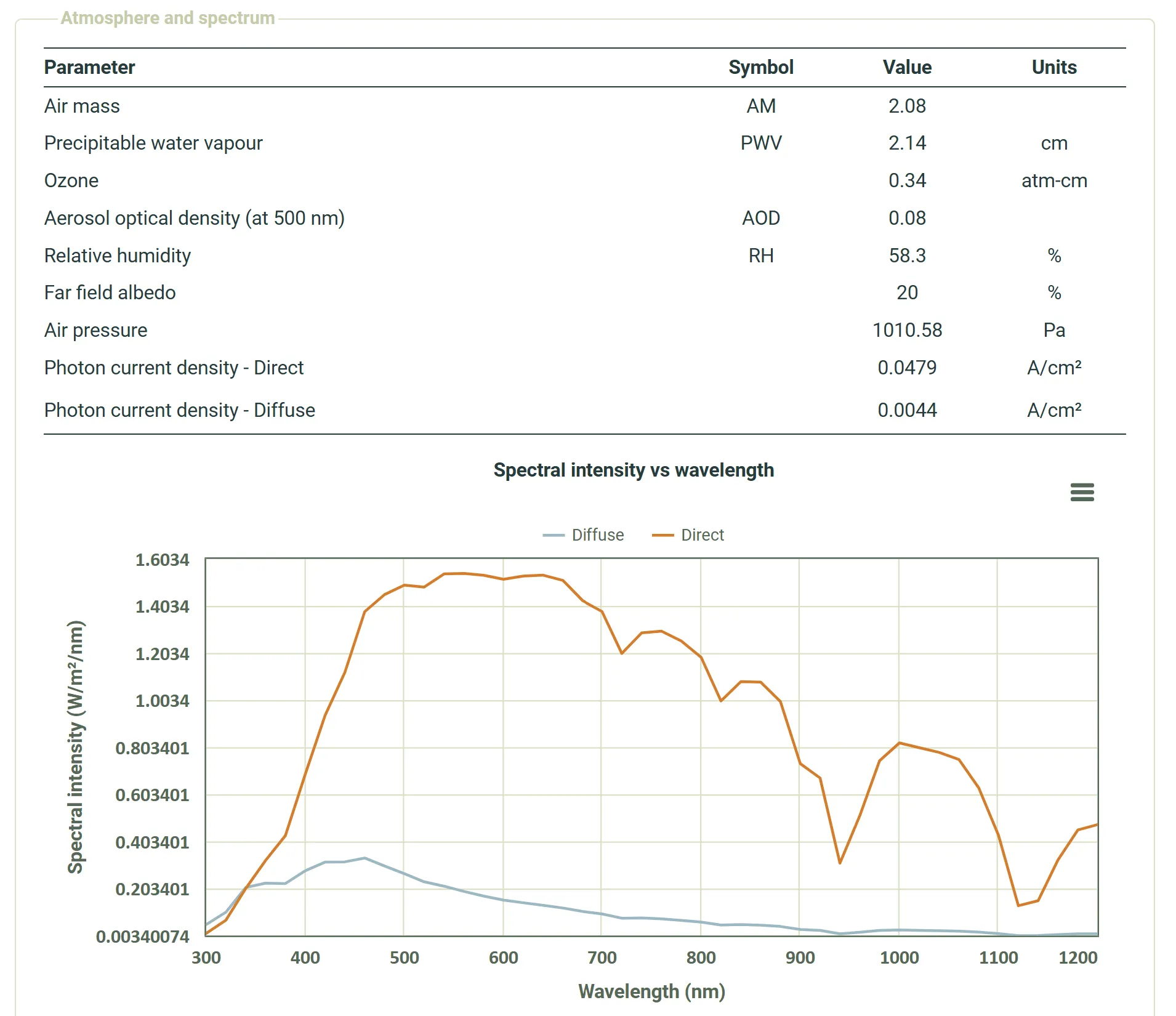
Section titled “Retrieve hourly data and examine detailed results”Sometimes it is useful to examine simulation results at a finer level of detail. SunSolve allows you to retrieve data for a single day and view conditions on an hourly basis. This includes detailed cell-level heat maps showing light absorption, along with the spectral distribution of direct and diffuse irradiance at that time.
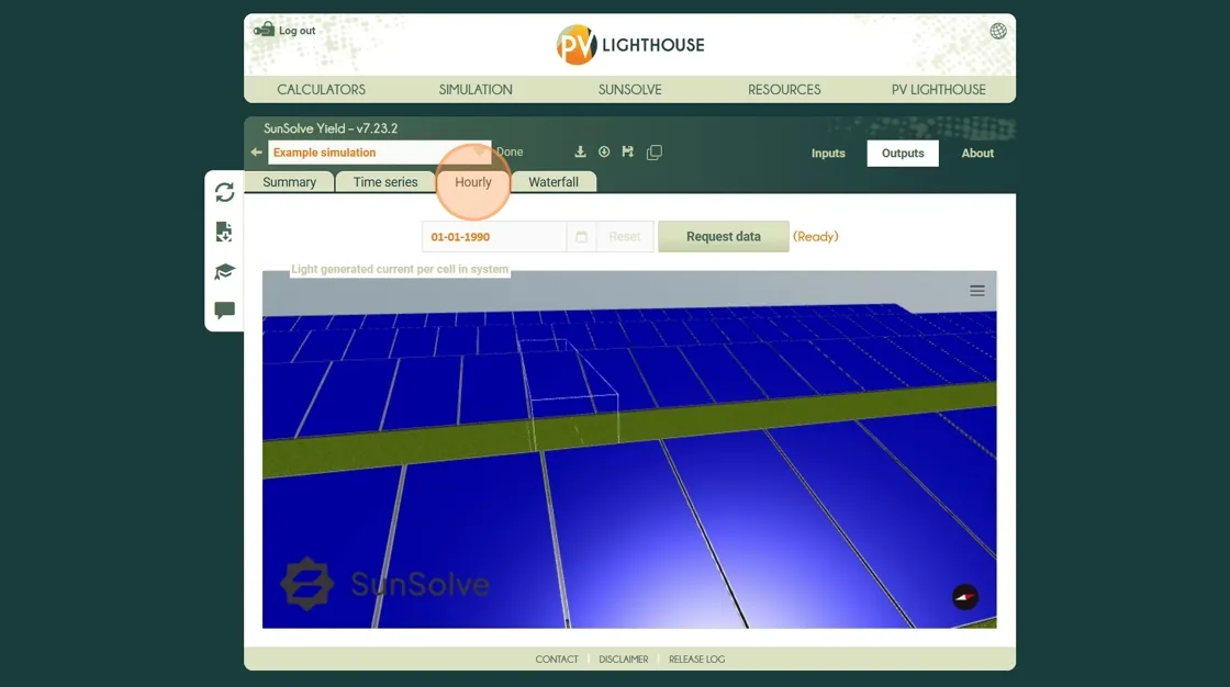
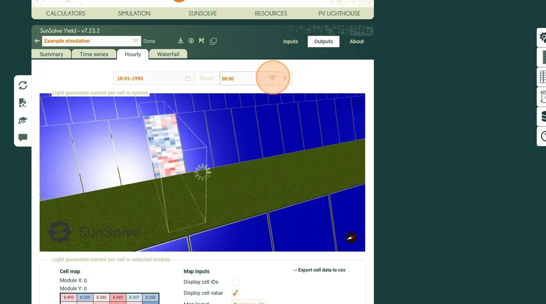
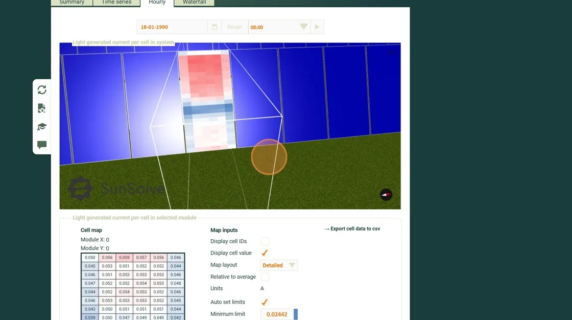
Step 11. Click Time step viewer to open the time step data workspace. Note in earlier versions of SunSolve this tab was called Hourly.
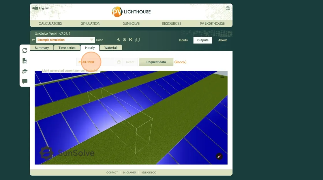
Step 12. Click the Select Date field.
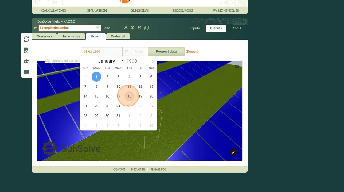
Step 13. Select day 18 to view results for January 18th.
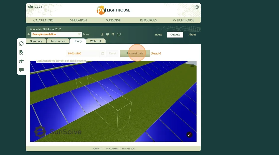
Step 14. Click Request data. Once the data is loaded, you can select an hour to display.
Step 15. Choose 08:00 to examine the system at 8 a.m. on January 18th. A heat map appears, showing the per-cell absorption pattern across the module.
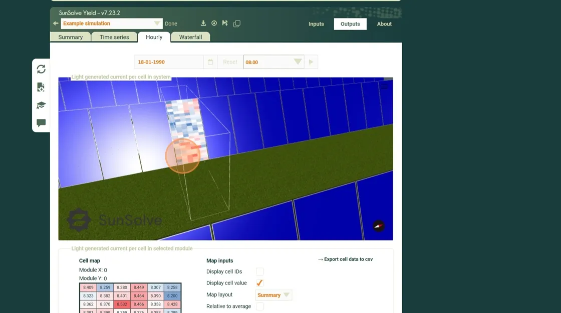
Step 16. Click and drag to rotate the view, use the mouse wheel to zoom, and hold Ctrl while dragging to pan horizontally or vertically.
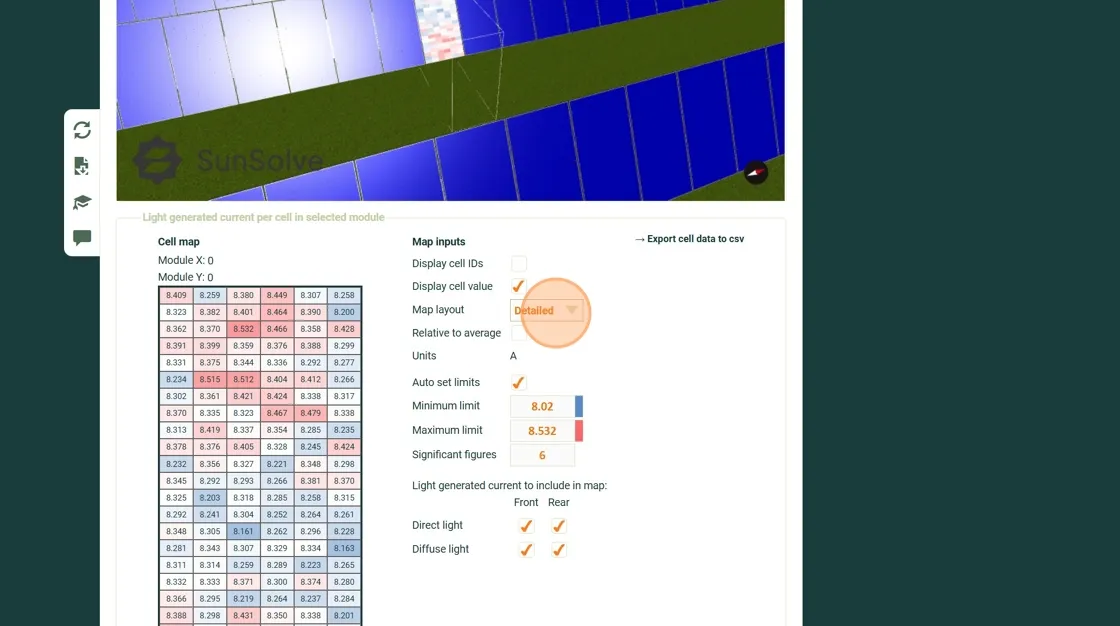
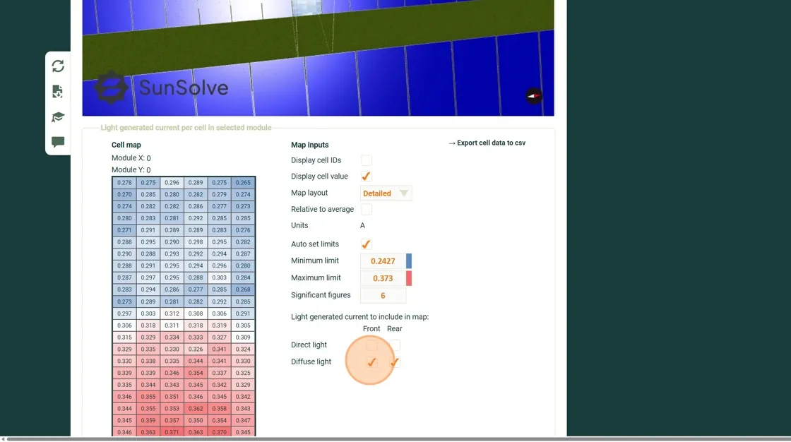
Step 17. Scroll down and select Detailed to reveal additional options for light-generated current components.
Step 18. Deselect the Front and Rear direct light options. The cell heat map now displays absorption from diffuse light only.
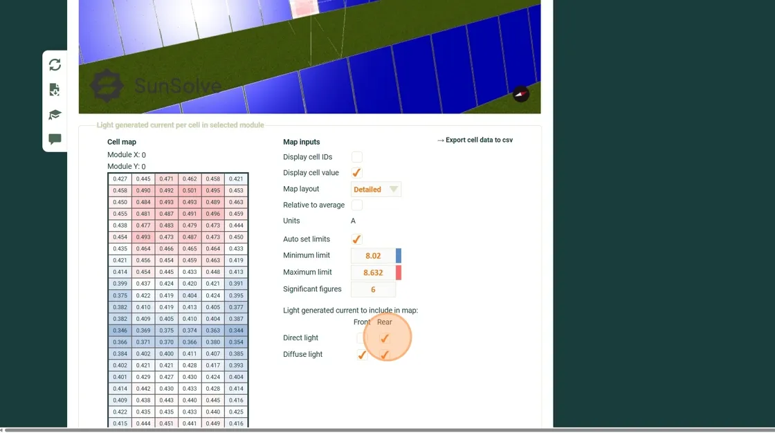
Step 19. Scroll back up to the 3D view of the system. Now you can see the distribution in cell current from diffuse light. The top of the panel receives more light and thus appears more red.
Step 20. Return to the detailed panel and deselect Diffuse Front. The cell heat map now shows absorption on the rear side due to diffuse light only. Note that the pattern appears identical when viewed from either direction.
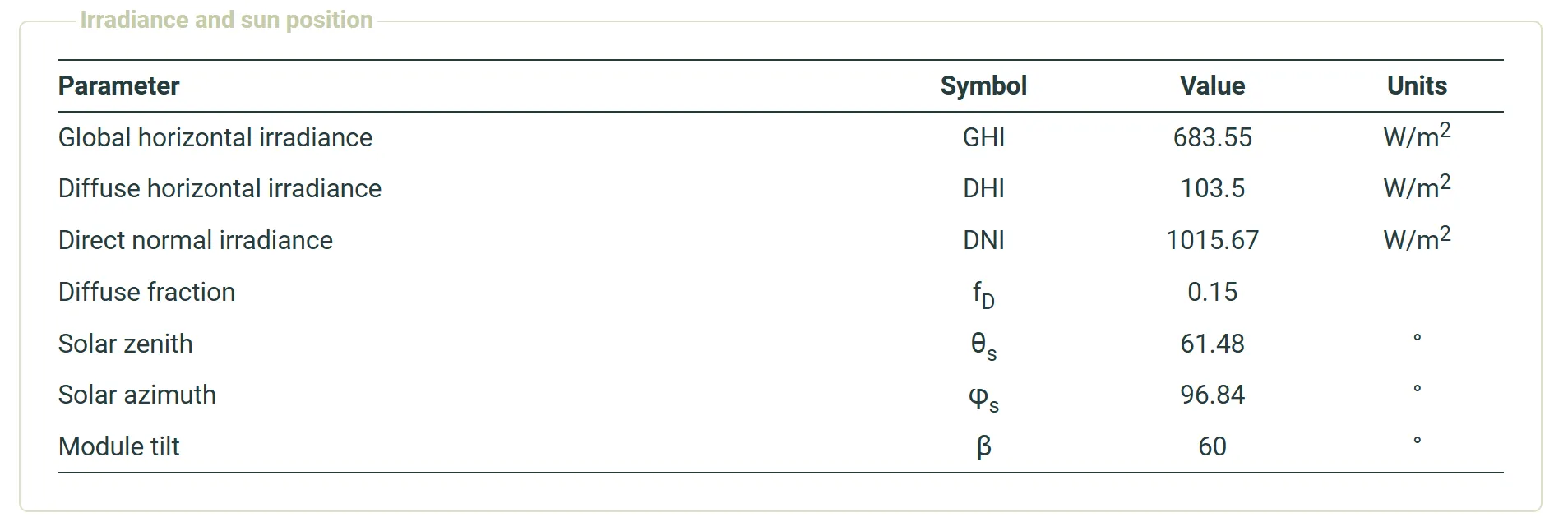
Step 21. Scroll to the bottom of the page to view detailed information about the weather, atmospheric conditions, and spectral distribution of direct and diffuse light at the selected hour.
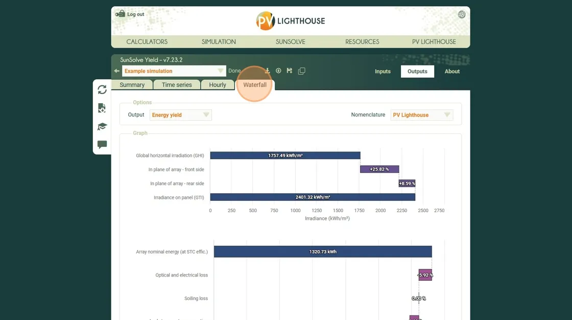
Waterfall chart of losses
Section titled “Waterfall chart of losses”SunSolve provides a progressive breakdown of the optical, thermal, and electrical losses within the system using a waterfall-style chart. Each bar in the chart represents a stage in the energy flow — from incident sunlight to the DC output of the modules. This helps identify which processes contribute most to performance losses, such as optical shading, temperature effects, or electrical mismatch. The upper section of the chart displays the irradiation components, showing how the in-plane irradiation on the front and rear sides compares with the global horizontal irradiation (GHI). The lower section presents the energy yield chain, beginning with the array’s nominal energy under standard test conditions (STC) and applying successive losses until the final DC yield is reached.
Step 22. Click Waterfall loss to open the loss analysis view.
Step 23. To export the data behind the chart, click → Download summary data.
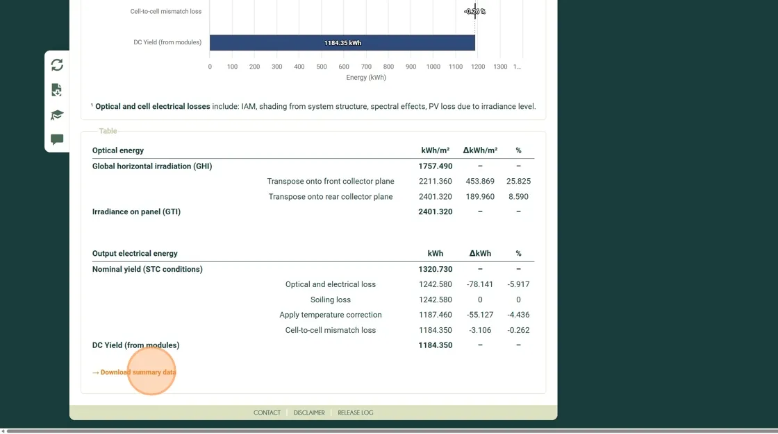
In this simple example, the waterfall chart concludes with the DC Yield of the modules. For full system simulations, additional stages such as inverter conversion losses, wiring effects, and AC output will also be included.
Summary
Section titled “Summary”You’ve now learned how to explore, interpret, and export simulation results in SunSolve Yield — from viewing time-series and hourly data to examining detailed per-cell absorption and Waterfall loss charts.
The next tutorial covers saving and reloading simulations, so you can manage, duplicate, and revisit your projects for ongoing analysis.