Equivalent circuit model

SunSolve Yield models the electrical behaviour of photovoltaic cells using an equivalent circuit approach. Each solar cell is represented by a circuit that includes a current source for the light-generated current, linked to the ray-tracing results. The circuit also includes diodes and resistors that represent the different loss mechanisms within a solar cell.

This circuit is widely used in yield modelling to calculate the electrical output of cells and modules under a wide range of operating conditions.

A key difference in SunSolve Yield is that this model is applied at the cell level. Many other yield programs apply the model at the module level, a simplification that speeds up solving but removes the ability to resolve cell-level effects, such as electrical mismatch.

Current density vs. current notation

The equivalent circuit parameters in SunSolve are entered and stored as current densities (denoted J, with units of A/cm²) normalised by the cell area. This approach allows for direct comparison between cells of different sizes and simplifies parameter extraction from measured data.

In the equations presented on this page, currents are written using I notation (amperes) for consistency with standard circuit analysis conventions. The relationship between current density and current is:

$$I = J \times A_{\text{cell}}$$

Where A_cell is the active area of the solar cell in cm². For example:

• I_L = J_L × A_cell (light-generated current)
• I₀₁ = J₀₁ × A_cell (saturation current)

Similarly, resistances scale inversely with area. The specific resistances (entered in Ω·cm²) are divided by cell area to obtain the circuit resistances (in Ω):

• Circuit resistance: R_s (Ω) = Rs (Ω·cm²) / A_cell (cm²), where Rs is the specific series resistance parameter
• Circuit resistance: R_sh (Ω) = Rsh (Ω·cm²) / A_cell (cm²), where Rsh is the specific shunt resistance parameter

During simulation, SunSolve applies this scaling internally for each cell based on its geometry.

Simplified equivalent circuit model

The most commonly used equivalent circuit model for the solar cell is shown in the figure below. In this case the circuit is limited to the use of a single diode (i.e. the n=2 diode and resistive limited enhanced recombination components are disabled).

This model is compatible with other programs (such as PVsyst) and is a required assumption when using the PVsyst temperature model.¹

Simplified single-diode equivalent circuit model for a solar cell.

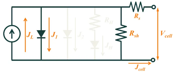
The IV characteristics are determined using the following equations:

$$I = I_L - I_0 \left[ \exp \left( \frac{q(V + IR_s)}{nkT} \right) - 1 \right] - \frac{V + IR_s}{R_{sh}}$$

Where I₀ , n, R_s, and R_sh are the circuit inputs for saturation current, ideality factor, series resistance and shunt resistance; all defined at a nominal temperature (typically 25°C). I_L is the light generated current which is linked to the result of the ray tracing. The symbols q, k, and T represent the elementary charge, Boltzmann constant, and absolute temperature (in Kelvin), respectively.

Full equivalent circuit model

SunSolve also supports a more comprehensive equivalent circuit model that includes additional diode and recombination components, as shown below.

Full equivalent circuit model with multiple diode components.

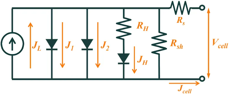
The full model includes:

• First diode: Saturation current I₀₁ with ideality factor m₁ ≈ 1.

• Second diode: Saturation current I₀₂ with ideality factor m₂ ≈ 2.

• Resistive-limited enhanced recombination component: Saturation current I_0H with ideality factor m_H and series resistance R_H.

When all components are enabled, the full IV equation becomes an implicit set of equations that must be solved numerically:

$$I = I_L - I_{01} \left[ \exp \left( \frac{q(V + IR_s)}{m_1kT} \right) - 1 \right] - I_{02} \left[ \exp \left( \frac{q(V + IR_s)}{m_2kT} \right) - 1 \right] - I_H - \frac{V + IR_s}{R_{sh}}$$

where the current through the resistive-limited component is:

$$I_H = I_{0H} \left[ \exp \left( \frac{q(V_H)}{m_HkT} \right) - 1 \right]$$

and the voltage across the H diode is:

$$V_H = V + IR_s - I_HR_H$$

Note that only the current I_H flows through the resistance R_H, not the total cell current I.

Notes:

• the full equivalent circuit model is only available to Advanced Users.
• this model is not compatible with standard temperature correction models which assume a single diode.
• the implementation in SunSolve assumes no temperature dependence of the additional diodes.

Optional circuit components

Illumination-dependent shunt resistance

Optionally an irradiance-dependent shunt resistor may be defined. This model is more applicable to non-crystalline silicon devices and in modern high efficiency modules can likely be neglected in most cases. Note that it is unclear how the inclusion of this model impacts the reverse bias behaviour if included simply to match the low light behaviour of the max power point.

$$R_{sh} = R_{sh,inf} + (R_{sh,0} - R_{sh,inf}) \times \exp \left( -R_{sh,exp} \times \frac{G}{G_{ref}} \right)$$ $$R_{sh,inf} = \frac{R_{sh,ref} - R_{sh,0} \times exp(-R_{sh,exp})}{1 - exp(-R_{sh,exp})}$$

Where G is the irradiance, G_ref is the reference irradiance (typically 1000 W/m²), R_sh,0 is the shunt resistance at zero irradiance, R_sh,ref is the shunt resistance at the reference irradiance and R_sh,exp is the exponent.

For a discussion of the relevance and implications of this model, see Illumination-Dependent Shunt Resistance in c-Si Module Models.

Voltage- and illumination-dependent loss component

Optionally, a voltage- and illumination-dependent recombination loss term may be included in the equivalent circuit. This component is primarily used for thin-film solar cells, particularly amorphous silicon (a-Si:H) and cadmium telluride (CdTe) devices, where photocurrent exhibits non-superposition behaviour and significant forward-bias roll-off.

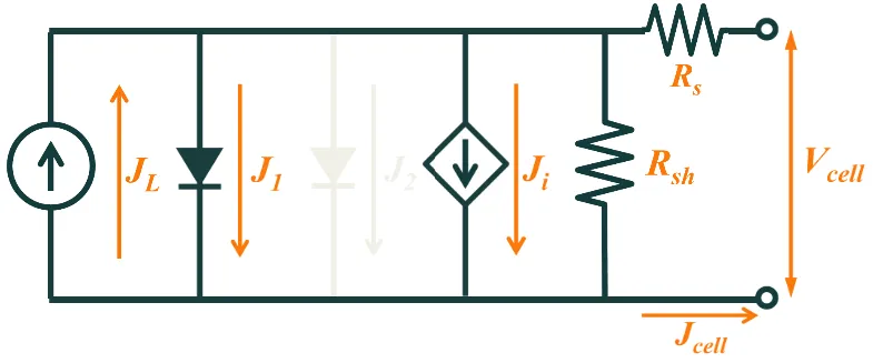
Equivalent circuit model with voltage- and illumination-dependent recombination loss component.

The loss current is given by:

$$I_{\text{rec}} = \frac{I_L \cdot d_i^2 / (\mu \tau_{\text{eff}})}{V_{\text{bi}} - V}$$

Where $I_L$ is the light-generated current (linking the loss to illumination intensity), $d_i^2 / (\mu \tau_{\text{eff}})$ is a combined material parameter representing the i-layer thickness squared divided by the effective minority carrier mobility-lifetime product, V_bi is the built-in voltage, and V is the internal voltage across the diode junction (equal to V_terminal + IR_s).

This term represents recombination losses that increase under both higher illumination (via I_L) and forward bias (as the internal junction voltage V approaches V_bi). The denominator captures the reduction in internal electric field strength as forward bias reduces the effective depletion width.

When enabled, the full cell current–voltage equation becomes:

$$I = I_L - I_{\text{rec}} - I_0 \left[ \exp \left( \frac{q(V + IR_s)}{nkT} \right) - 1 \right] - \frac{V + IR_s}{R_{sh}}$$

In the numerical implementation, smooth regularisation functions are applied near the singularity at V = V_bi to ensure robust convergence in the circuit solver (SunSolve uses a SPICE-based solver for all equivalent circuit calculations).

This component is typically disabled for crystalline silicon modules, where superposition holds and diode recombination dominates.

Note:

• In practice, the parameter $d_i^2 / (\mu \tau_{\text{eff}})$ is typically fitted to measured IV curves rather than calculated from the individual physical properties it represents.
• While this loss component was originally developed for a-Si devices, and the equation parameters reflect that origin, it has also been successfully applied to CdTe devices.
• The recombination current is numerically capped at 99% of I_L to prevent unphysical solutions.

Module-level equivalent circuit parameters

While SunSolve Yield performs all circuit calculations at the cell level, the user interface also displays equivalent circuit parameters scaled to the module level. This presentation facilitates comparison with other yield modelling programs (such as PVsyst) that work exclusively at the module level.

The conversion from cell-level to module-level parameters depends on the electrical topology of the module, specifically the number of cells connected in series within each string (N_series) and the number of strings connected in parallel (N_parallel).

Reverse saturation currents

The reverse saturation currents (I₀₁, I₀₂, I_0H) scale with the total active area of cells connected in parallel:

$$I_{0,\text{module}} = J_{0,\text{cell}} \times N_{\text{parallel}} \times A_{\text{cell}}$$

Where J_0,cell is the cell-level current densities (A/cm²) and A_cell is the active area of a single cell (cm²).

Resistances

The series and shunt resistances scale according to the series-parallel arrangement:

$$R_{\text{module}} = R_{\text{cell}} \times \frac{N_{\text{series}}}{N_{\text{parallel}} \times A_{\text{cell}}}$$

Where R_cell is the cell-level specific resistance (Ω·cm²) as entered in the user interface.

This scaling reflects that:

• Series connection multiplies resistance by the number of cells in the string
• Parallel connection divides resistance by the number of strings
• The cell-level specific resistance must be divided by cell area to obtain the circuit resistance

Voltage-dependent recombination parameter

For the voltage- and illumination-dependent recombination loss component described above, the material parameter $d_i^2 / (\mu \tau_{\text{eff}})$ scales only with the series-parallel topology:

$$\left( \frac{d_i^2}{\mu \tau_{\text{eff}}} \right)_{\text{module}} = \left( \frac{d_i^2}{\mu \tau_{\text{eff}}} \right)_{\text{cell}} \times \frac{N_{\text{series}}}{N_{\text{parallel}}}$$

This scaling ensures that the voltage dependence of the recombination loss remains physically consistent when applied at the module level.

Ideality factors

The ideality factors (m₁, m₂, m_H, n) are dimensionless quantities that do not change between cell and module levels.

Note: These module-level values are provided for reference and comparison with other tools. All yield simulations within SunSolve are performed using the cell-level parameters to preserve the ability to resolve electrical mismatch and other cell-level effects.

Implementation details

Determination of cell light generated current

The light generated current within each cell is calculated at every time step using the following procedure. Note that the calculations are performed in terms of current density (J in A/cm²), which is then scaled by cell area to obtain the total current I_L used in the circuit equations.

1. The wavelength dependent photon count for the direct and isotropic components of incident irradiance are adjusted based on the selected sky model.

2. The wavelength dependent absorption within the cell is calculated for the specific sun position based on the linear interpolation of the nearest three solar angles.

3. At each wavelength the four components of light generated current are calculated as:

   $$J_{L,front,direct} = \cos(\text{zenith}) \cdot J_{Ph,normal}(\lambda) \cdot A_{front,direct}(\lambda) \cdot SF_{front}(\lambda)$$ $$J_{L,rear,direct} = \cos(\text{zenith}) \cdot J_{Ph,normal}(\lambda) \cdot A_{rear,direct}(\lambda) \cdot SF_{rear}(\lambda)$$ $$J_{L,front,diffuse} = J_{Ph,isotropic}(\lambda) \cdot A_{front,isotropic}(\lambda) \cdot SF_{front}(\lambda)$$ $$J_{L,rear,diffuse} = J_{Ph,isotropic}(\lambda) \cdot A_{rear,isotropic}(\lambda) \cdot SF_{rear}(\lambda)$$

   Where SF is the wavelength dependent scaling factor that is applied to simple modules based on their quantum efficiency and STC value of front and rear I_SC (as described in Module current scaling). For complex modules this is not required.

4. The final value for the light generated current density at the nominal temperature (i.e., 25 °C) is the sum of the above four components, giving J_L. This is then multiplied by the cell area to obtain I_L for use in the circuit equations.

The value is subsequently adjusted based on the module temperature as outlined below.

Determination of the series resistance

SunSolve offers two approaches for determining the series resistance R_s used in the equivalent circuit:

Option 1: Fixed series resistance value

The user provides a single value for R_s that applies to all cells. This approach is appropriate when electrodes are not explicitly modelled or when a simplified resistance model is sufficient.

Option 2: Analytical grid resistance calculation

The user provides the non-grid series resistance R_s,1 and SunSolve calculates the grid resistance R_s,2 analytically based on electrode geometry and material properties. The total series resistance is:

$$R_s = R_{s,1} + R_{s,2}$$

This approach is available when electrodes are enabled and provides a more detailed representation of series resistance for complex module designs. The analytical calculation accounts for:

1. The geometry of the cell, including the shape, dimensions and thickness.

2. The resistivity of the main absorbing substrate.

3. The sheet resistance between electrode fingers on the front and rear sides.

4. The contact resistance between the electrode fingers and the substrate, including calculation of the transmission length to account for the strength of the sheet resistance underneath the contact.

5. The shape, layout and resistivity of the fingers, busbars and ribbons.

6. The additional length of ribbons used to connect to the next cell.

The equations are based on the approach of calculating the power loss in the components when operating under maximum power point conditions and then converting that into a resistive value. The general approach along with many of the equations is described in the textbook by Professor Green [Green1982]. When using the analytical approach an additional amount of series resistance (R_s,a) may be added to account for other components that are not included in the equations, such as the module connectors.

For more detail on how SunSolve applies these equations, see the relevant section of the SunSolve Power manual.

Temperature dependence of electrical circuit

The temperature dependence of the equivalent circuit inputs is determined using the PVsyst circuit temperature model [Mermoud2014]. Input values for J_L, I₀, and n are adjusted according to the following:

$$I_L(T) = I_{L,nominal} \cdot \left( 1 + \left( \frac{\mu_L}{100} \right) \cdot (T - T_{nominal}) \right)$$ $$I_0(T) = I_{0,nominal} \cdot \left( \frac{T}{T_{nominal}} \right)^3 \cdot \exp \left[ \frac{q E_G}{nk} \cdot \left( \frac{1}{T} - \frac{1}{T_{nominal}} \right) \right]$$ $$n(T) = n_{nominal} \cdot \left( 1 + \left( \frac{\mu_n}{100} \right) \cdot (T - T_{nominal}) \right)$$

Where μ_L and μ_n are inputs to the model that represent the change in I_L and n measured in %/°C and T_nominal is the specified reference temperature for I_L, I₀, and n (typically 25°C).

Footnotes

1. The reasons for this are somewhat historical and relate to the fact that module IV outputs provided on a typical datasheet limit the number of outputs that can be measured and subsequently fitted. By including these extra circuit components there are too many input parameters that require fitting to too few outputs. This problem can be resolved with a matrix of temperature dependent IV curves and a complex curve fitting algorithm to determine the full set of inputs. ↩