Modifiers

Modifiers are part of the electrical solver and allow SunSolve Power users to adjust equivalent-circuit input parameters (J_L, J₀, m, R_s and R_sh) on a per-cell basis within a module. This feature enables modelling of non-uniform conditions such as partial shading, cell degradation, manufacturing variations, and localized defects. Modifiers are only available for simulations with a Device configuration set to Unit-module or Module (not for single-cell configurations). This feature cannot be loaded into SunSolve Yield.

What are modifiers?

Each modifier applies a fractional (multiplicative) change to one or more equivalent-circuit parameters for specific cells or groups of cells. Where multiple circuits are used, each modifier applies to a single circuit. Rather than defining absolute parameter values, modifiers use multipliers where:

• 1.0 = 100% = no change (default)
• 1.1 = 110% = 10% increase
• 0.9 = 90% = 10% decrease
• 2.0 = 200% = doubling the parameter
• 0.5 = 50% = halving the parameter

For example, a J_L multiplier of 0.2 applied to a cell reduces its light-generated current to 20% of its original value, simulating 80% shading.

When to use modifiers

Modifiers enable modelling of non-uniform module conditions that commonly occur in real-world installations. Common applications include:

• Partial shading: Simulate shadows, soiling, or snow coverage by reducing J_L
• Non-uniform illumination: Model varying light intensity across cells (sometimes easier than defining multiple overlapping illumination sources)
• Cell degradation: Adjust multiple parameters simultaneously (e.g., increased J₀₁, decreased J_L, increased R_s)
• Manufacturing variations: Represent parameter differences between cell batches
• Hot spots: Reduce R_sh to model micro-cracks or localized damage
• Bypass diode studies: Create intentional current mismatch to analyze bypass diode behavior

Modifiers should be applied to a module simulation after the optical solving has been run. They do not affect the optical result, only the electrical output. It is possible to add and edit the modifiers on a simulation without the need to rerun the ray tracer. The user interface will detect the change to the electrical model and will rerun the electrical solver as needed.

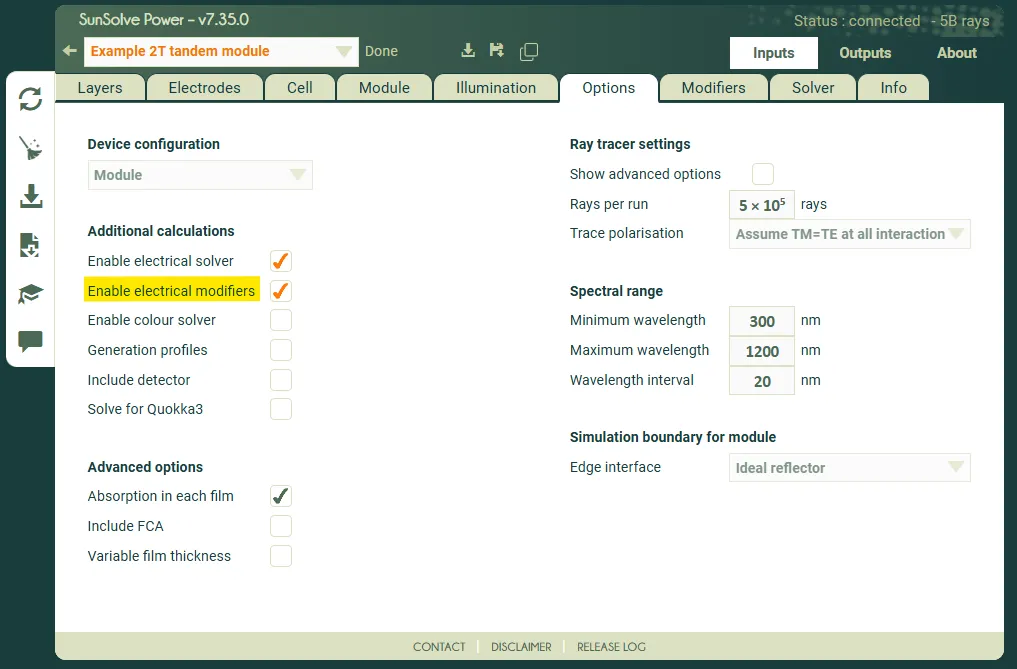
Configuring modifiers

To use modifiers you must first enable them on the Inputs -> Options tab. They are only available for the module based device configurations and only appear when the electrical solver is active.

Once enabled, modifiers are configured on the Inputs -> Modifiers tab. A new modifier is added using the + Add equivalent circuit modifier button. There is no limit to how many modifiers can be added to a single simulation. They appear in a list in the order they were added and are applied in that order during calculation.

The screenshot below shows an example where three modifiers have been added. The title of each indicates the cell, circuit and input parameters that are modified.

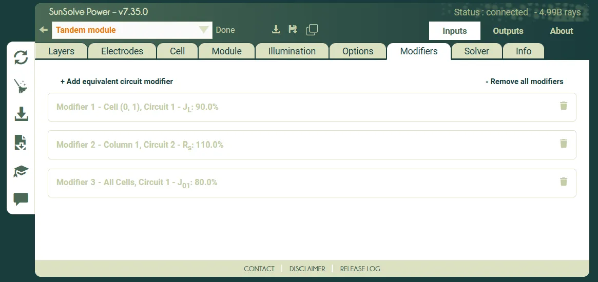
To edit the details of any modifier simply click on the summary text to expand the window.

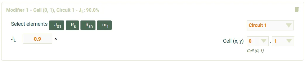
Each modifier has two main sections: one for adding and editing specific parameters and another for defining the target circuit and cell.

Parameter multipliers

The inputs required to select and edit modifiers for specific equivalent-circuit inputs are located on the left side of the panel. Select which parameters to adjust by clicking the green buttons next to Select elements. This list will only show buttons for input parameters that are enabled in that circuit (i.e. on the Inputs -> Cell tab), and not already added as a parameter to this specific modifier. Once selected they will appear with a text box to enter the multiplier value. You may select as many parameters as needed.

Enter multiplier values in the input fields. To remove a parameter, click the × button next to it.

Cell and circuit targeting options

The inputs required to define the sub-circuit and cell within the module to which the modifiers apply are located on the right of the panel.

Circuit: For multi-junction (tandem) cells with multiple circuits, you must select which specific circuit the modifier should affect. The modifier will only be applied to that specific sub-circuit.

Cell Position: Enter X and Y coordinates to target specific cells or cell groups:

• All: Apply to all cells in the row or column (default)
• Set both X and Y: Apply to a specific cell at position (X, Y)
• Set only X: Apply to all cells in column X (entire vertical column)
• Set only Y: Apply to all cells in row Y (entire horizontal row)

Note: cell positions use zero-based indexing where (0, 0) is the bottom-left cell.

Managing modifiers

• Remove single modifier: Click the trash icon in the modifier’s summary bar
• Remove all modifiers: Click - Remove all modifiers
• Disable temporarily: Uncheck Apply modifiers on the Inputs -> Options tab to disable all modifiers without deleting them

Note: It is not necessary to rerun the optical solver when adding, removing, or changing modifiers. They can be edited at any time after optical solving is complete and the electrical solver will automatically rerun.

Practical example: Individual cell shading

Simulate shading on specific cells of a 144 half-cut cell module:

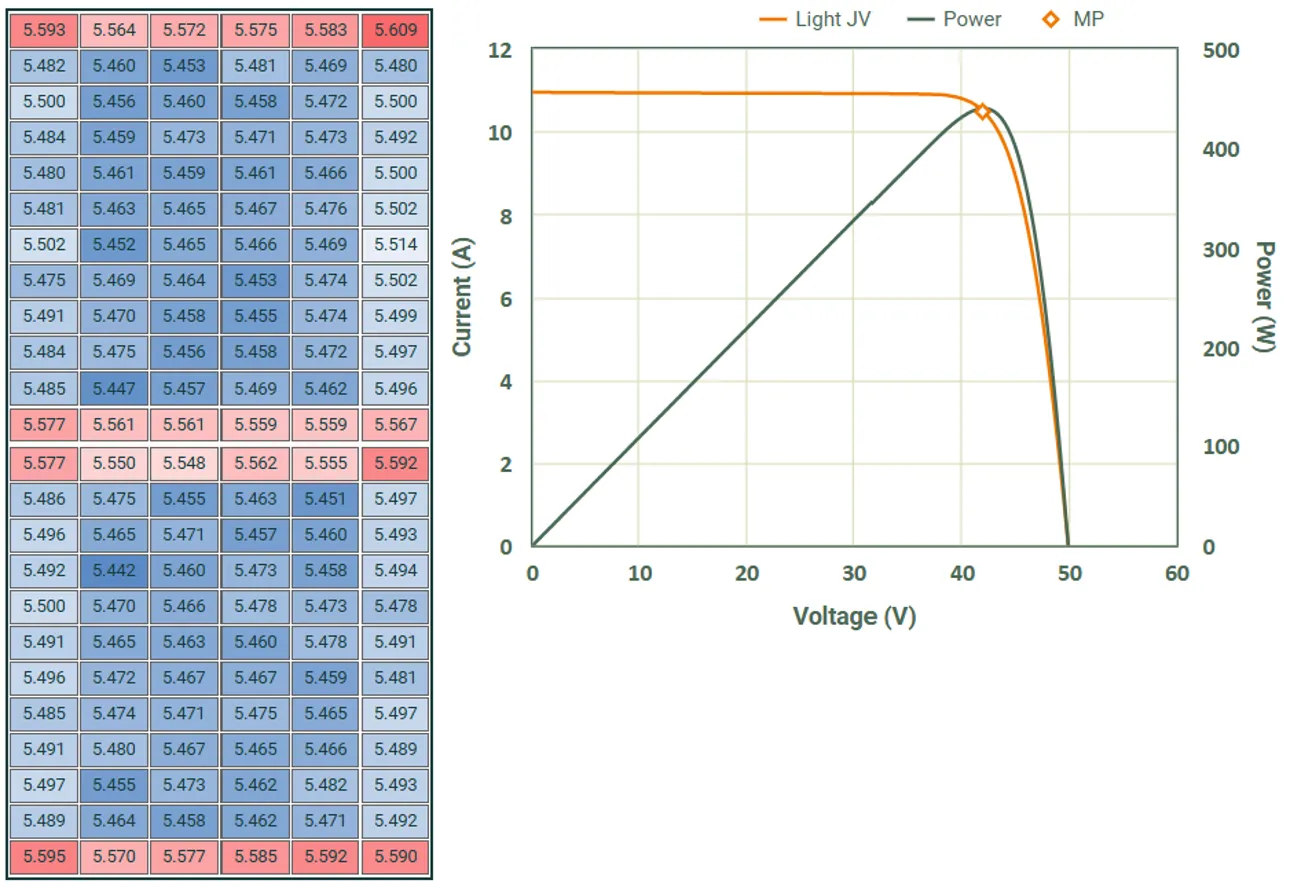
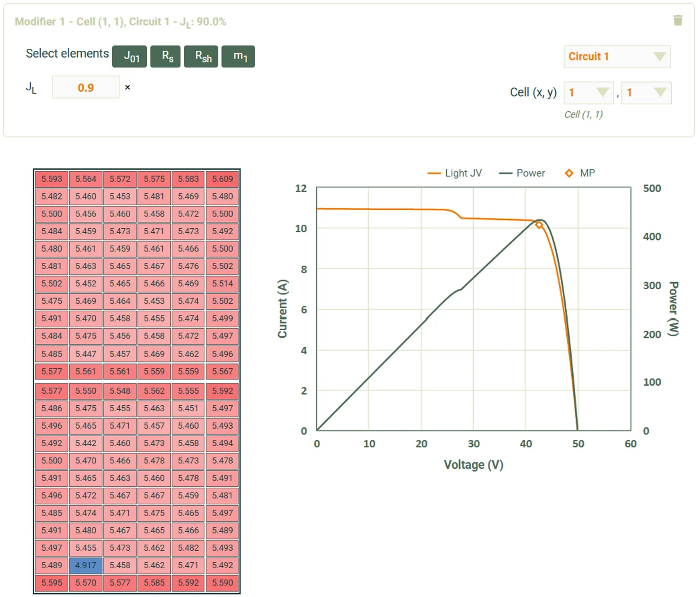
1. Create the module and solve the optical model. The cell map and IV curve are shown below.

2. Add a new modifier:
   • Add J_L parameter with multiplier 0.9 (10% light reduction)
   • Set cell positions: X=1, Y=1 (lower-left)
   • The electrical output will update to reflect the reduction in cell current and its impact on the IV curve

3. Add a second modifier:
   • Add J_L parameter with multiplier 0.8 (20% light reduction)
   • Set cell positions: X=5, Y=11 (middle-right)
   • Now there are two cells shaded

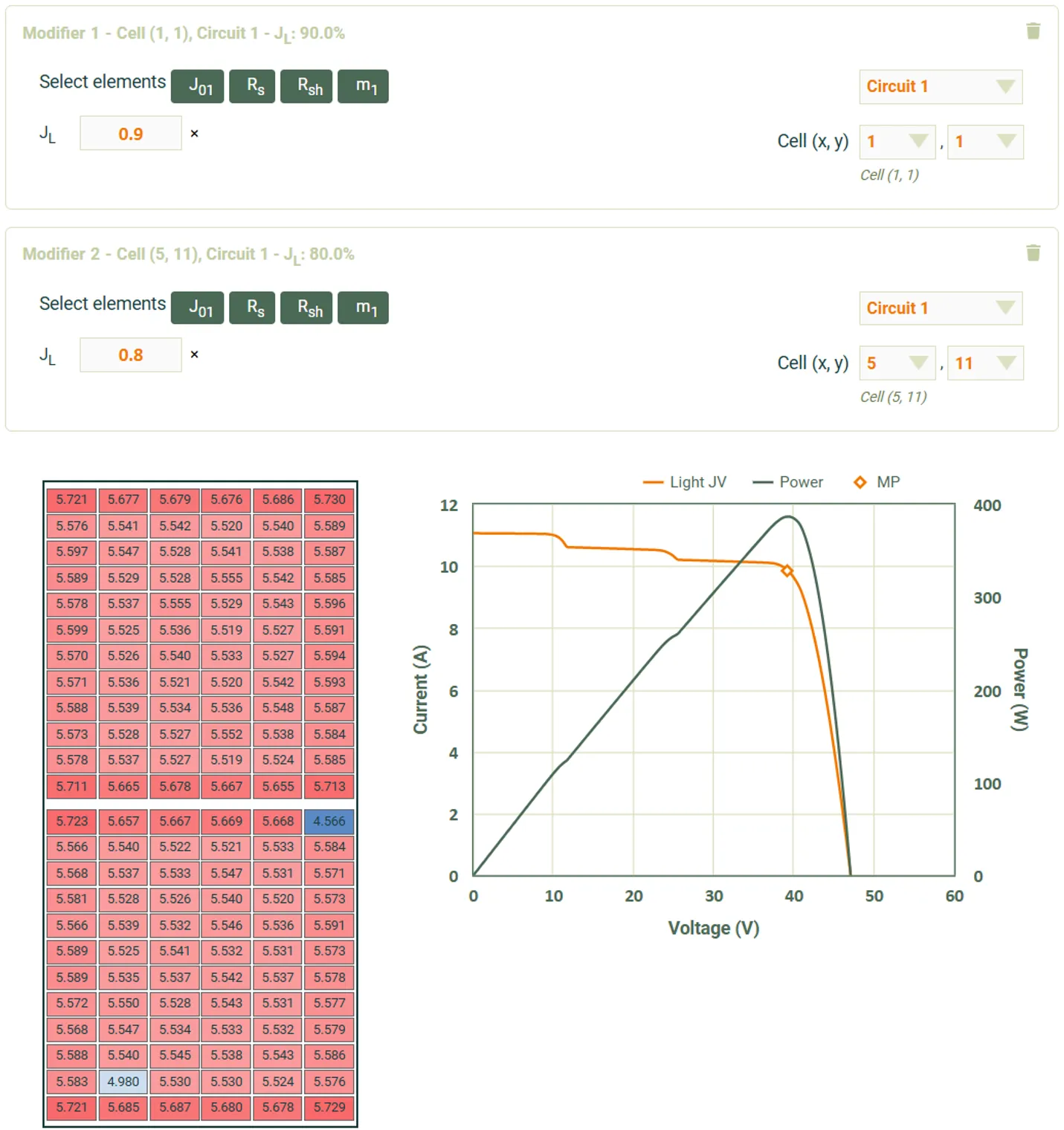
With these modifiers applied, the two targeted cells have their J_L reduced to 90% and 80% of the optical values respectively, while all other cells remain unaffected. The current-limiting effect in the strings containing these cells creates characteristic steps in the IV curve and reduces maximum power output due to increased mismatch losses.

Important limitations and considerations

Sweep and optimisation interaction

For a simulation that uses the solve type Sweep, the full list of modifiers is applied to every sweep condition. It is not possible to sweep the values of the modifiers themselves.

Simulations that use the solve type Optimisation will apply the modifiers to every run within every generation.

Multipliers, not absolute values

Modifiers use multiplicative changes only. You cannot set absolute values directly. To achieve a specific parameter value, you must calculate the required multiplier from the base value.

Example: If base R_s = 0.5 Ω·cm² and you want R_s = 0.6 Ω·cm², use multiplier 0.6 / 0.5 = 1.2.

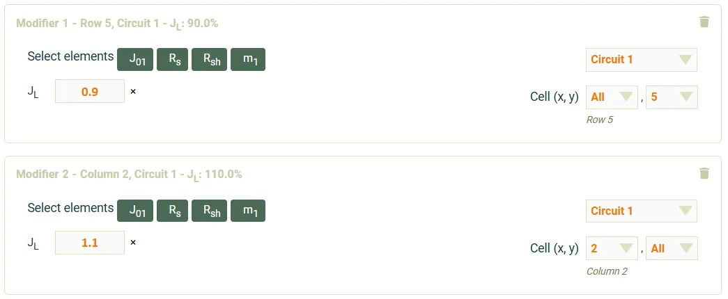
Multiple modifiers may impact the same cell

If two or more modifiers are set to impact any specific cell, then all will be applied, in the order they appear in the modifier list. For example, in the screenshots below the first modifier reduces the J_L of every cell in the row 5 to 90%. The second modifier then increases the J_L of every cell in the column 2 to 110%

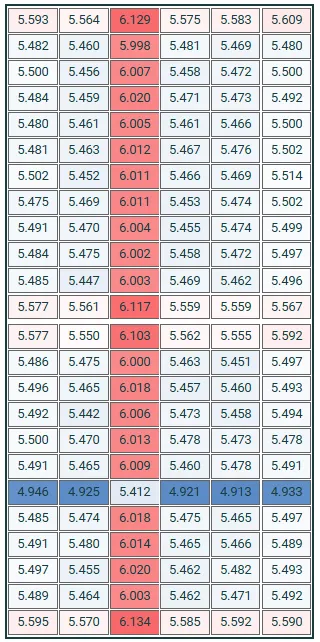
The resulting cell map demonstrates that the overlap cell at (2, 5) is affected by both modifiers. In this case it is close to unaffected; however the value is slightly reduced since 0.9 * 1.1 = 0.99.

Temperature interaction

Modifiers are applied at T_nominal (the reference temperature where equivalent-circuit parameters are defined, typically 25°C) before temperature correction to T_operating. This means:

• Multipliers are applied to parameters at the nominal/reference temperature (typically 25°C)
• After applying modifiers, temperature coefficients are used to correct parameters from T_nominal to T_operating
• The final solve at T_operating uses temperature-corrected versions of the adjusted parameters
• Modifiers should represent conditions at T_nominal, as they are defined relative to the reference temperature

Related topics

• Main solving algorithms - Overall solving process including where modifiers fit
• Cell and module layout - Understanding cell positioning for targeting
• Solver modes - Sweeping modifier multipliers for sensitivity analysis