
Inputs - Modifiers
Modifiers are part of the electrical solver and allow SunSolve Power users to adjust equivalent-circuit input parameters (JL, J0, m, Rs, Rsh, VB1, JB1, VB2, JB2, VBH and JBH) on a per-cell basis within a module.
This feature enables modelling of non-uniform conditions such as partial shading, cell degradation, manufacturing variations, and localised defects, as well as the statistical spread of cell performance across a batch of modules.
Modifiers are only available for simulations with a Device configuration set to Unit-cell module or Module.
This page is an overview of the feature. The modifiers tab offers three workflows, each documented on its own page:
- Single module applies exact adjustments to chosen cells of one module.
- Module population (distributions) samples many modules from parameterised statistical distributions.
- Module population (measured cells) builds many modules from an imported file of measured cells.
What are modifiers?
Section link: What are modifiers?Each modifier applies a fractional (multiplicative) change to one or more equivalent-circuit parameters for specific cells or groups of cells. Where multiple sub-circuits are used (i.e. in tandem devices), each modifier applies to a single sub-circuit. Rather than defining absolute parameter values, modifiers use multipliers where:
1.0= 100% = no change (default)1.1= 110% = 10% increase0.9= 90% = 10% decrease2.0= 200% = doubling the parameter0.5= 50% = halving the parameter
For example, a JL multiplier of 0.2 applied to a cell reduces its light-generated current to 20% of its original value, simulating 80% shading.
When to use modifiers
Section link: When to use modifiersModifiers enable modelling of non-uniform module conditions that commonly occur in real-world installations. Common applications include:
- Partial shading: Simulate shadows, soiling, or snow coverage by reducing JL
- Non-uniform illumination: Model varying light intensity across cells (sometimes easier than defining multiple overlapping illumination sources)
- Cell degradation: Adjust multiple parameters simultaneously (e.g., increased J01, decreased JL, increased Rs)
- Manufacturing variations: Represent parameter differences between cell batches
- Hot spots: Reduce Rsh to model micro-cracks or localised damage
- Reverse bias breakdown variation: Adjust VB1/JB1, VB2/JB2, or VBH/JBH to model cells with different breakdown characteristics on any enabled diode, for example to study the impact of weak cells on hot-spot risk under partial shading
- Bypass diode studies: Create intentional current mismatch to analyse bypass diode behaviour
Modifiers should be applied to a module simulation after the optical solving has been run. They do not affect the optical result, only the electrical output. It is possible to add and edit the modifiers on a simulation without the need to rerun the ray tracer. The user interface will detect the change to the electrical model and will rerun the electrical solver as needed.
Enabling modifiers
Section link: Enabling modifiersTo use modifiers you must first enable them on the Inputs → Options tab. They are only available for the module-based device configurations and only appear when the electrical solver is active.

Once enabled, modifiers are configured on the Inputs → Modifiers tab.
Ray tracing is required before modifiers
Section link: Ray tracing is required before modifiersModifiers are locked until the optics have been solved, because the electrical solve needs the ray-traced light-generated current (JL) as its baseline, and the fit to open-circuit voltage and fill factor is defined against that baseline. You cannot solve the electrical model without the optical result, so the modifier definition stays locked until ray tracing has run. This applies to all modifier workflows.
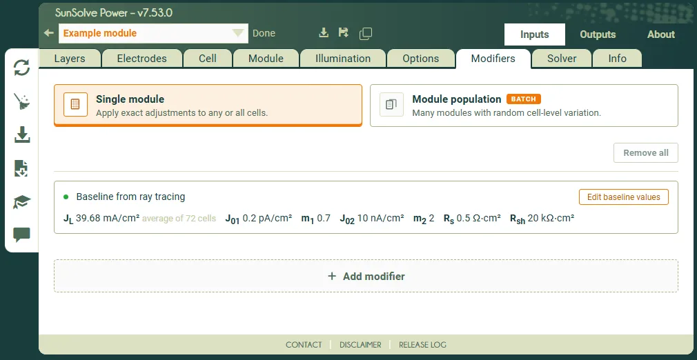
Until ray tracing has run, the panel shows “Please run ray tracing to enable modifiers.” Once it has run, the panel shows “Baseline from ray tracing” together with the baseline equivalent-circuit values for each circuit and an Edit baseline values action to edit them on the Inputs → Cell tab.
Choosing a scope
Section link: Choosing a scopeThe first choice on the Modifiers tab is the scope, which determines how many modules are built and how their cells are varied.
- Single module: applies exact adjustments to any or all cells of one module, producing a single realisation. Use this to study a specific pattern such as a named shaded cell, a degraded row, or a deliberate mismatch. See Single module.
- Module population: builds many modules whose cells vary from module to module, producing a distribution of module outputs rather than a single result. Use this to study manufacturing spread and the resulting mismatch-loss distribution. See the two population sources below.
Choosing a population source
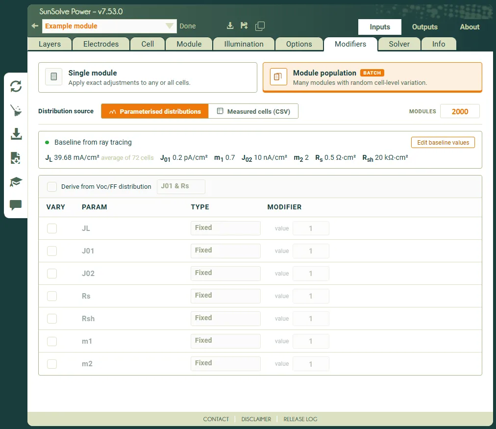
Section link: Choosing a population sourceWhen the scope is Module population, a Distribution source selector chooses where the per-cell variation comes from:
- Parameterised distributions: each parameter is drawn from a statistical distribution (fixed, Gaussian, top-hat or lognormal). You may also derive the distributions from a target open-circuit voltage and fill factor. See Module population (distributions).
- Measured cells (CSV): the cells are taken from an imported file of measured cell parameters, optionally binned to preserve realistic sort groups. See Module population (measured cells).
Whichever workflow you use, the results of a population run are read on the distribution results output page.
Important limitations and considerations
Section link: Important limitations and considerationsBase circuit
Section link: Base circuitModifiers scale per-cell copies of the equivalent circuits configured on the Inputs → Cell tab. Changing a base value changes the effective value produced by the same modifier, while disabled components cannot be modified or fitted. See How modifiers are applied for the calculation sequence.
Sweep and optimisation interaction
Section link: Sweep and optimisation interactionFor a simulation that uses the solve type Sweep, the full list of modifiers is applied to every sweep condition.
It is not possible to sweep the values of the modifiers themselves.
Simulations that use the solve type Optimisation will apply the modifiers to every run within every generation.
Multipliers, not absolute values
Section link: Multipliers, not absolute valuesModifiers use multiplicative changes only. You cannot set absolute values directly. To achieve a specific parameter value, you must calculate the required multiplier from the base value.
Example: If base Rs = 0.5 Ω·cm² and you want Rs = 0.6 Ω·cm², use multiplier 0.6 / 0.5 = 1.2.
Temperature interaction
Section link: Temperature interactionModifiers are applied at Tnominal (the reference temperature where equivalent-circuit parameters are defined, typically 25°C) before temperature correction to Toperating. This means:
- Multipliers are applied to parameters at the nominal/reference temperature (typically 25°C)
- After applying modifiers, temperature coefficients are used to correct parameters from Tnominal to Toperating
- The final solve at Toperating uses temperature-corrected versions of the adjusted parameters
- Modifiers should represent conditions at Tnominal, as they are defined relative to the reference temperature