Module cell layout

The module cell layout defines the physical geometry of the module and its cells. In SunSolve Yield, this geometry is configured in the Layout tab of the module popover, which appears when you load or preview a module.

SunSolve Yield supports two module types, each with different layout inputs:

• Simple module — the active region is treated as a uniform rectangular block with user-specified dimensions. No individual cell geometry is defined. This is the faster option and is suitable when detailed optical modelling of the cell structure is not required.
• Complex module — individual cells are arranged in a grid with configurable spacing, grouping, and perimeter. This provides full 3D optical modelling of the cell layout.

Both module types use the same electrical circuit layout, which is configured separately in the Circuit tab.

Simple module layout

For a simple module, the layout inputs define the overall physical dimensions of the active area:

• Width ($X_M$) — the module width in cm
• Height ($Y_M$) — the module height in cm
• Thickness ($Z_M$) — the total module thickness in cm

The active region is modelled as a uniform block with optical properties defined by a surface lookup table rather than individual cell and layer definitions. See Simple module optics for details of the optical model.

The number of cells in the X and Y directions is still defined for the simple module. These values determine the electrical circuit layout (the number of cells in each string) and the per-cell area, which is calculated as the total active area divided by the number of cells. Although the optical geometry of the module is unchanged, a different cell count alters how the ray-traced absorption is distributed across cells, which can affect stochastic error.

Complex module cell layout

For a complex module, the layout inputs mirror those available in SunSolve Power and control the detailed physical arrangement of cells within the module. Cells are arranged in a grid, with the bottom-left cell labelled as X=0, Y=0. Columns and rows are always aligned.

Cell layout

The cell layout inputs define how many cells the module contains and how they are arranged in the grid. All values are adjusted using increment/decrement buttons rather than free-text entry.

Columns

The number of columns of cells in the module.

Rows

The number of rows of cells in the module.

Total number of cells

A read-only output calculated as columns multiplied by rows.

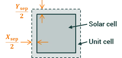
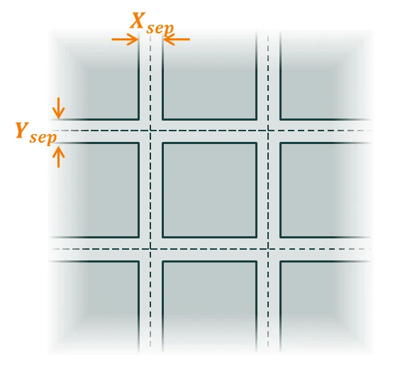
Cell spacing

Cell spacing defines the gap between adjacent cells. This space is filled by the same layer materials (e.g., encapsulant and backsheet) as defined on the Layers tab, and directly affects the optical simulation — light entering the cell gap region interacts with the inter-cell materials rather than the active cell area.

The figure below shows how the user inputs, $X_{\text{sep}}$ and $Y_{\text{sep}}$, define the distance between the edge of the solar cell and the edge of the unit cell. (The solar cell and the unit cell are concentric.)

Cell groups

When Define cell groups is enabled, the module’s cells are divided into groups with additional spacing between them. This is a purely optical input — it adds extra inter-cell gap material between groups of cells without changing the electrical circuit topology.

Cell groups are useful for modelling modules where physical gaps exist between blocks of cells, such as half-cut cell modules with a gap along the centreline, or modules with visible spacing between cell groups for aesthetic reasons.

When cell groups are enabled, the following inputs appear:

• Groups per row — the number of cell groups in the X direction
• Groups per column — the number of cell groups in the Y direction
• X separation ($X_g$) — the extra spacing between groups in the X direction (only shown when groups per row > 1)
• Y separation ($Y_g$) — the extra spacing between groups in the Y direction (only shown when groups per column > 1)

The group spacing $X_g$ and $Y_g$ is in addition to the standard cell spacing. It does not add extra space to the module perimeter.

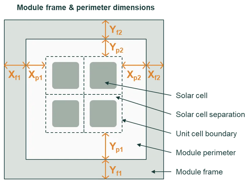
Module perimeter

When Include perimeter is enabled, additional space is added around the outermost cells of the module. This perimeter region uses the same layer structure as the inter-cell gap. Four values can be set independently:

• Left ($X_{p1}$), Right ($X_{p2}$), Bottom ($Y_{p1}$), Top ($Y_{p2}$)

The perimeter is distinct from the frame, which sits outside the active module area. The perimeter defines the gap between the outermost cells and the frame (or module edge if no frame is present). The layers, materials, and interfaces within the perimeter region are the same as those within the cell-separation region of the unit cells, as defined on the Layers tab.

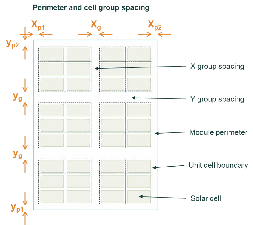
The figure below shows a module with 4 cells in each row and 9 cells in each column, grouped into 2 cell groups in the X direction and 3 cell groups in the Y direction. It illustrates how the cell group spacing, perimeter, and frame dimensions relate to each other.

Standard layouts

SunSolve provides preset standard module layouts that can be loaded to quickly configure common module configurations. These presets set the cell count, spacing, and arrangement to match widely used module designs. Standard layouts are available when the inputs are not locked.

Calculated module dimensions

The module preview section at the top of the module popover displays computed dimensions and areas based on the geometry inputs. All areas are in cm² and dimensions in cm.

Single cell area

The area of one cell, as determined by the cell shape and dimensions.

Total cell area

The combined active area of all cells in the module:

$$A_{\text{total cell}} = A_{\text{cell}} \times N_x \times N_y$$

where $N_x$ and $N_y$ are the number of columns and rows.

Cell gap area

The total area of non-cell regions inside the module perimeter — the inter-cell spacing, any cell group spacing, and any perimeter white space. This is the area filled by the encapsulant and backsheet layers. For a simple module this value is zero.

Frame area

Only shown when a frame is included. The total area occupied by the frame material around the module perimeter:

$$A_{\text{frame}} = (F_{x1} + F_{x2}) \times Y_{\text{inner}} + (F_{y1} + F_{y2}) \times X_{\text{inner}} + F_{x1} F_{y1} + F_{x1} F_{y2} + F_{x2} F_{y1} + F_{x2} F_{y2}$$

where $X_{\text{inner}}$ and $Y_{\text{inner}}$ are the dimensions inside the frame (cells + spacing + perimeter) and $F_{x1}$, $F_{x2}$, $F_{y1}$, $F_{y2}$ are the frame widths on each side.

Module area

The overall footprint of the module:

$$A_{\text{module}} = X_{\text{total}} \times Y_{\text{total}}$$

X dimension and Y dimension

The overall module dimensions. For a complex module these are built up from the cell and spacing inputs:

$$X_{\text{total}} = N_x \times (W_{\text{cell}} + X_{\text{sep}}) + (G_x - 1) \times X_g + X_{p1} + X_{p2} + F_{x1} + F_{x2}$$ $$Y_{\text{total}} = N_y \times (H_{\text{cell}} + Y_{\text{sep}}) + (G_y - 1) \times Y_g + Y_{p1} + Y_{p2} + F_{y1} + F_{y2}$$

where $G_x$ and $G_y$ are the number of cell groups (1 if cell groups are disabled), $X_g$ and $Y_g$ are the group spacings, $X_{p1}$/$X_{p2}$/$Y_{p1}$/$Y_{p2}$ are the perimeter values (0 if perimeter is disabled), and $F_{x1}$/$F_{x2}$/$F_{y1}$/$F_{y2}$ are the frame widths (0 if no frame).

For a simple module, the X and Y dimensions are directly entered as $X_M$ and $Y_M$ (plus any frame widths if a frame is included).