Simulating spatially varying albedo and reflective groundsheets
This tutorial shows how to model non-uniform ground reflectivity in SunSolve Yield — from a simple uniform albedo baseline through to reflective groundsheets and non-uniform dirty ground patches. By the end, you will be able to set up scenes with multiple ground materials of different reflectance, compare the effect on rear-side irradiance, and represent a dirty groundsheet as a degraded-reflectance scenario.
Setting up a baseline simulation with uniform albedo
Section titled “Setting up a baseline simulation with uniform albedo”Before introducing spatially varying ground conditions, establish a baseline with a single uniform ground material. This gives you a reference point for comparing the effect of any ground modifications.
System setup
Section titled “System setup”- Create a new simulation using the Tracking bifacial system template and open it. See Running your first simulation for a walkthrough of template selection and project setup.
Setting the ground albedo
Section titled “Setting the ground albedo”-
Navigate to Inputs > System and find the Ground > Albedo section. The ground surface is configured using the reflector library — see Ground albedo for a full reference on reflector selection, scaling factor, and effective albedo display.
-
The default template uses Vegetation > Green grass with a scaling factor of 1. For this tutorial, change the ground surface to use the soil material described below in Configuring a soil material.
-
Run the simulation. See Running your first simulation if you are unfamiliar with running simulations.
-
Once the simulation completes, open the Outputs workspace and record the bifacial performance ratio () from the Summary tab as your baseline reference value.
The baseline output represents the rear-side irradiance contribution from a perfectly uniform ground surface. All subsequent modifications will be compared against this result.
Configuring a soil material
Section titled “Configuring a soil material”Several steps in this tutorial require configuring a surface to use a soil material. The process is the same whether you are setting the ground albedo or the material of a custom object (dirt patch):
- Set the material mode to Custom and click → Show details to open the surface details dialogue. See Surface details dialogue for a full reference on this dialogue.
- Under Reflector RAT, select Wavelength dependent mode, then choose from the library: Soil > Brown to dark brown sand.
- Under Scattering, set the Lambertian fraction to 1 (100% diffuse reflection).
- Close the dialogue.
This material configuration is used for both the ground albedo baseline and the dirt patches on custom objects throughout this tutorial.
Adding a reflective groundsheet beneath the array
Section titled “Adding a reflective groundsheet beneath the array”Reflective groundsheets (such as white PVC strips) are increasingly used to boost rear-side irradiance in bifacial systems. In SunSolve, these are modelled using custom objects placed on the ground surface via the CAD Objects tab.
Adding the custom object
Section titled “Adding the custom object”- Navigate to Inputs > System and select the CAD Objects tab. Add a new custom object — see Custom objects for a full reference on object properties, positioning, and layout options.
Positioning and sizing the groundsheet
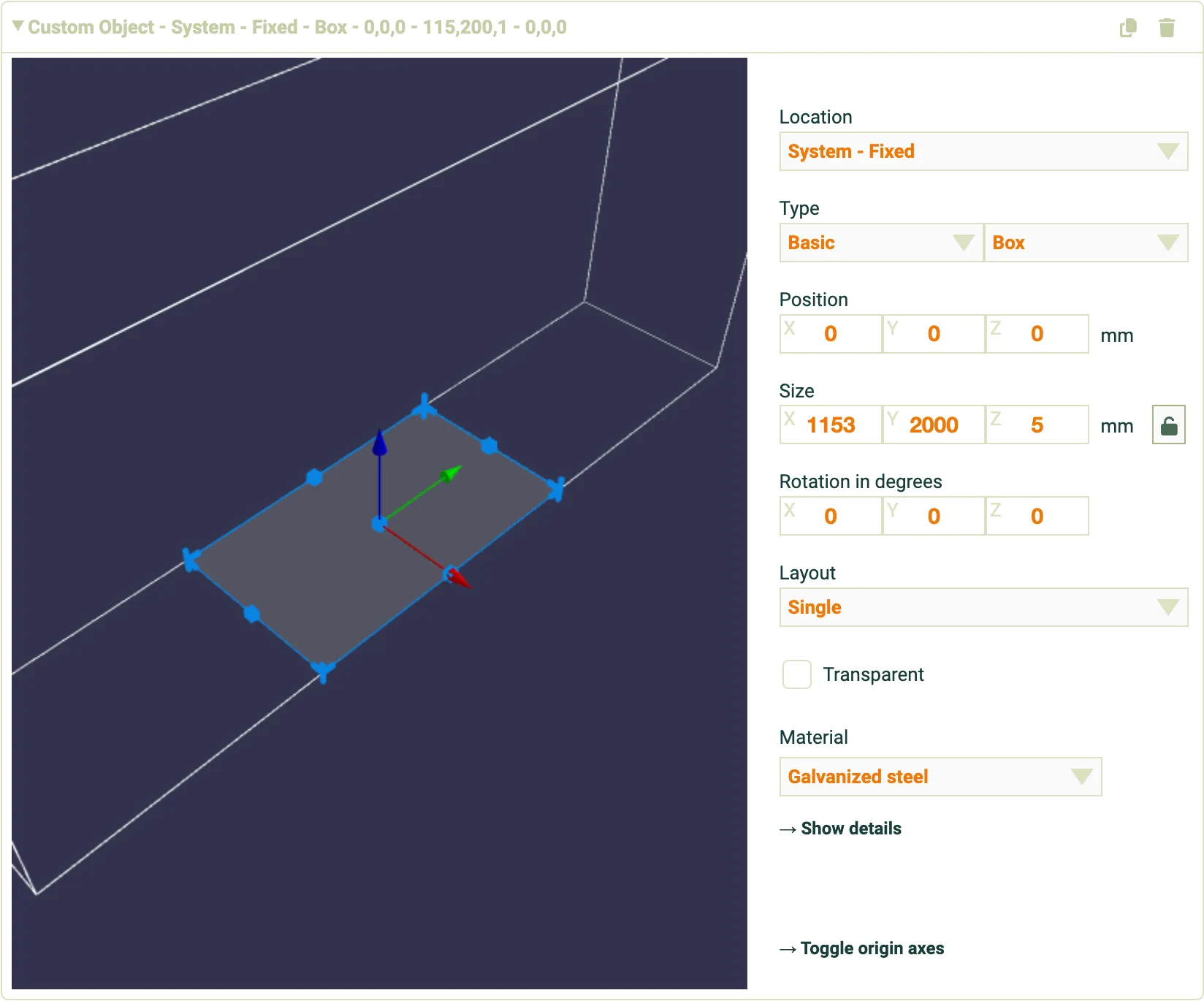
Section titled “Positioning and sizing the groundsheet”- Configure the object as a ground-level reflective groundsheet:
- Location: System - Fixed (the strip stays on the ground and does not track with the modules)
- Type: Basic > Box
- Position: Set Z to 0 so the groundsheet sits on the ground. Adjust X and Y to centre it beneath the tracker row.
- Size: Set X (width across the row) to match the unit system width from the Layout tab — in this example, 1153 mm. Set Y (length along the row) to 2000 mm to represent a 2 m groundsheet of white PVC material beneath the tracker. Set Z (height) to a small value such as 5 mm — the groundsheet should be essentially flat on the ground. Unlock the size lock icon for independent control of each dimension.
- Layout: Single.
Configuring reflection properties
Section titled “Configuring reflection properties”-
Change the Material dropdown to Custom, then click → Show details to open the material properties dialogue. For details on how material selection works, see Custom objects — Material.
-
Under Reflector RAT, change the mode to Constant with wavelength. Set R (reflectance) to 0.85 and A (absorptance) to 0.15 to represent a white PVC groundsheet. Under Scattering, leave the distribution set to Lambertian (100% diffuse reflection).
-
Close the material dialogue.
Running the simulation and comparing results
Section titled “Running the simulation and comparing results”-
Run the simulation with the reflective groundsheet in place.
-
View the results and compare against the baseline:
- Summary — Compare the bifacial performance ratio () and energy yield. An increase in indicates the reflective groundsheet is boosting rear-side contribution.
- Timestep viewer — View the colour-mapped 3D visualisation of light-generated current per cell. Cells above the reflective groundsheet should show higher current than the surrounding area.
- Time series data — Export per-cell or POA irradiance data as CSV for side-by-side comparison. See Time series data for details on output modes.
- Analysis tab — Review the PVSyst correction factors (, ) on the Inputs > Analysis tab. See Extracting bifacial factors for a full explanation of these factors.
The gain in rear-side irradiance depends on the groundsheet width, reflectance, and position relative to the module. Wider groundsheets with higher reflectance produce a larger effect.
Representing a dirty groundsheet as a degraded-reflectance scenario
Section titled “Representing a dirty groundsheet as a degraded-reflectance scenario”Reflective groundsheets degrade over time as dust, dirt, and organic material accumulate on their surface. You can use the same custom object setup to represent different levels of groundsheet dirtiness by varying the reflectance value across simulation runs. This is a quick sensitivity study you can run before modelling more complex non-uniform ground conditions.
Running dirty-groundsheet scenarios
Section titled “Running dirty-groundsheet scenarios”-
Set up a single reflective groundsheet object beneath the tracker row, as described in the earlier section.
-
Run three separate simulations, changing only the groundsheet’s reflectance value each time:
- Clean groundsheet: reflectance = 0.85
- Moderately dirty groundsheet: reflectance = 0.55
- Heavily dirty groundsheet: reflectance = 0.25
-
For each scenario, export the rear irradiance time series via Time series data using POA equivalent irradiance mode. Also record the energy yield and bifacial performance ratio from Viewing results for a quick high-level comparison.
Results comparison
Section titled “Results comparison”Record your simulation outputs in the following table to compare the three dirtiness levels:
Modelling non-uniform dirt on a groundsheet
Section titled “Modelling non-uniform dirt on a groundsheet”In practice, dirt does not accumulate uniformly across a groundsheet. Dust, organic debris, and other material build up unevenly — often concentrating near edges, joints, or areas with poor drainage — creating patches of reduced reflectance. SunSolve allows you to represent this by placing multiple custom objects with different sizes and layouts on top of the groundsheet.
The purpose of this type of modelling is to investigate the impact of non-uniform groundsheet dirtiness on rear irradiance, electrical mismatch, and specific yield — helping to quantify the value of cleaning or to compare different cleaning strategies (for example, determining the cost of leaving some dirt behind in hard-to-reach areas).
This section starts from the system configured in the previous section — with the white reflective groundsheet beneath the array and the ground albedo set to the soil material described in Configuring a soil material.
Adding the first dirt patch
Section titled “Adding the first dirt patch”-
On the CAD Objects tab, click + Add custom object to create a new object representing a dirt patch on the groundsheet.
-
Configure the object:
- Type: Basic > Box
- Size: Unlock the size lock icon, then set X = 400, Y = 800, Z = 8
- Position: X = -350, Y = -200, Z = 0
- Configure the material using the soil settings described in Configuring a soil material.
Duplicating and configuring the second dirt patch
Section titled “Duplicating and configuring the second dirt patch”-
Click the Duplicate icon (
 ) on the first dirt patch to create a copy that inherits its material properties.
 -
On the duplicated object, unlock the size lock icon again and configure:
- Size: X = 50, Y = 50, Z = 8
- Position: X = -200, Y = -800, Z = 0
- Layout: Repeated
- Objects: 20
- Distance between objects: X = 30, Y = 80, Z = 0
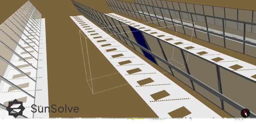
Viewing the result
Section titled “Viewing the result”- The 3D system image now shows the reflective groundsheet with a large dirt patch and a repeated array of smaller patches on its surface, all using the brown soil material.