
How to simulate plane-of-array irradiance
This guide shows how to record plane-of-array (POA) irradiance determined via SunSolve’s ray tracing engine. It does this by placing dedicated sensors into the 3D scene. These are specialised custom objects engineered to record irradiance on their front and rear surfaces uniformly at all wavelengths and incident angles.
The guide is dedicated to the POA irradiance measured across the whole module surface. The sensors used here are therefore always sized to match the module, rather than sampling a small area at a discrete point in the scene.
The tutorial steps through two key concepts that should be considered when simulating the POA irradiance.
- Measuring front and rear simultaneously versus measuring just one side.
- Measuring the average value across all modules in the unit-system versus measuring a single module.
Each step starts from the sensor built in the step before, so work through them in order.
- Measure the front and rear POA on every module.
- Measure the rear POA only, which is the configuration most people are looking for.
- Measure one specific module rather than the whole array.
Before you start
Section link: Before you startAll three steps are built on the same starting point. For these examples we will use the template for the 1P single-axis-tracker system. The weather is for the location of Sydney loaded from the PVGIS weather loader.
1. Create a new simulation
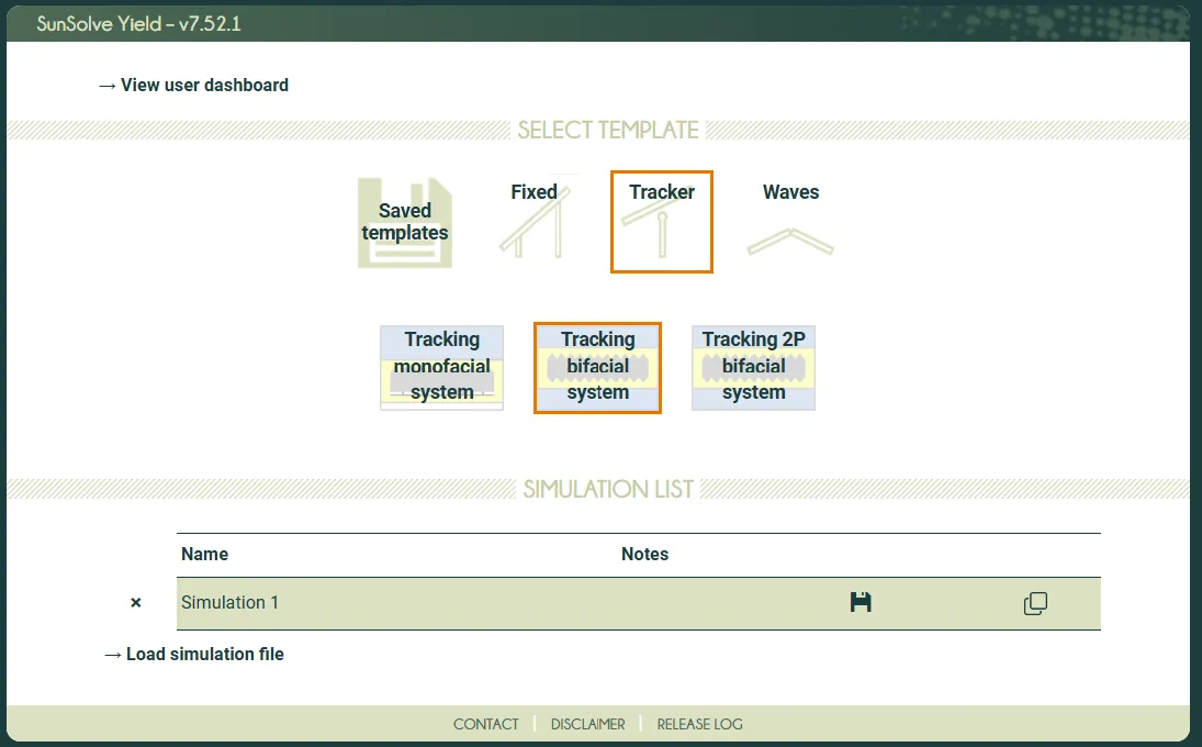
Section link: 1. Create a new simulationCreate a new 1P bifacial tracking simulation by clicking on the template shown in the screenshot below:
2. Load any weather file
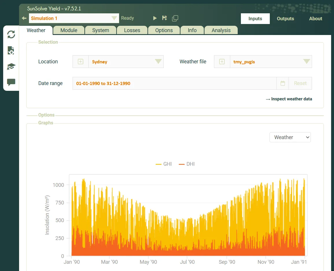
Section link: 2. Load any weather fileFor the examples shown here we are using a weather file for Sydney. You may load any weather that you would like to work with.
3. Select a module
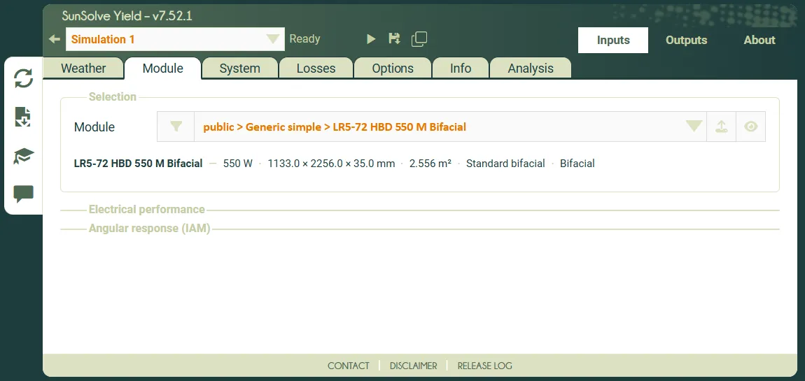
Section link: 3. Select a moduleFor the examples shown below we are using the LR5-72 module, a 550W panel from Longi.
Sensors, particularly where they are small relative to the scene, may require additional rays to be run (i.e. by turning up the simulation fidelity). This will minimise the stochastic noise in the irradiance. It is recommended that sensors should be the focus of the simulation, not obtaining results from high fidelity internal module optics. If it is desirable to have both, use two simulations: one in which the sensors are the focus and another optimised for the modules.
4. Set up the scene
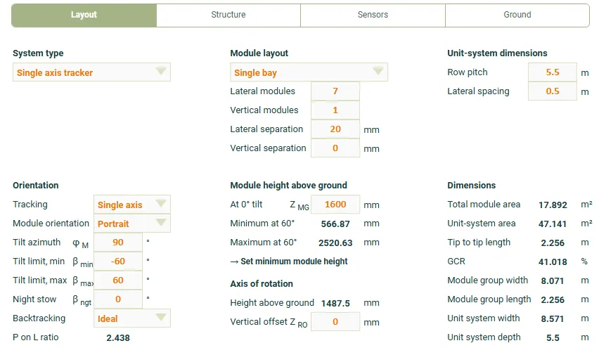
Section link: 4. Set up the sceneThis guide uses a scene representing a bay of seven modules with a post in the centre and small bay spacing at either end.
- Go to the Inputs > System tab and select the Layout sub-tab.
- Set Lateral modules to 7 modules.
- Set Lateral spacing to 0.5 m.
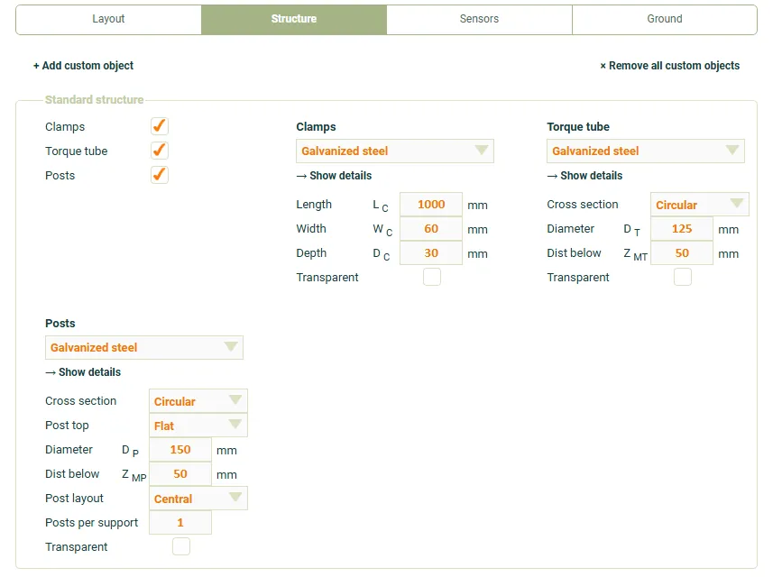
- From the Inputs > System tab, select the Structure sub-tab.
- Enable Posts.
5. Add a sensor to the scene
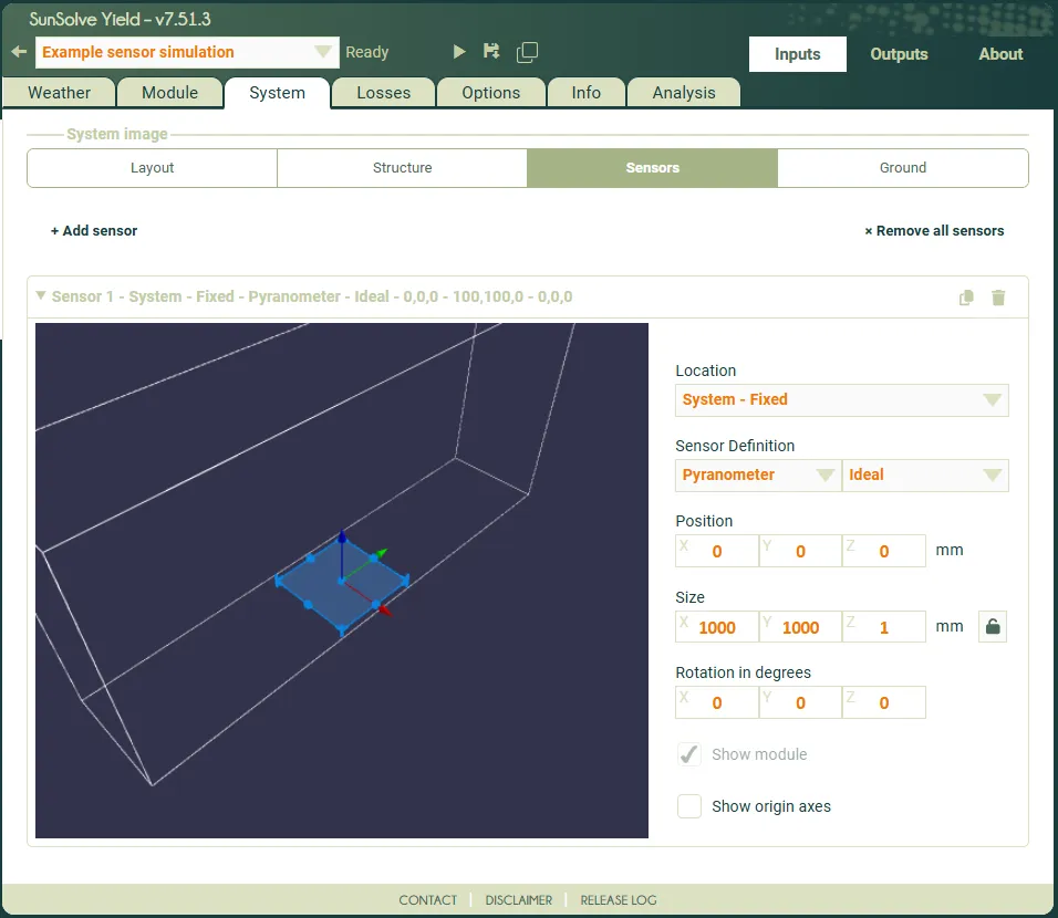
Section link: 5. Add a sensor to the scene- From the Inputs > System tab, select the Sensors sub-tab.
- Click + Add sensor.
You should see a sensor appear in the scene. The user interface will display a panel to edit that sensor. Note that you can minimise the larger system image at the top of the page to make the sensor’s inputs easier to see and access.
Step 1: measure front and rear POA on every module
Section link: Step 1: measure front and rear POA on every moduleThe first configuration places a sensor on every module in the scene. The sensor is positioned and sized such that its front and rear faces align with the front and rear faces of the module.
This provides an easy to use technique to record the full irradiance on the front and rear of every module in the scene. The results report the average irradiance on the module group.
Position the sensor over the module
Section link: Position the sensor over the module- Set the Location of the sensor to Module.
- Set the sensor Size to match the module dimensions in X, Y and Z.
- Add 2 mm to the Z dimension so the sensor face remains above the module surface at all rotation angles.
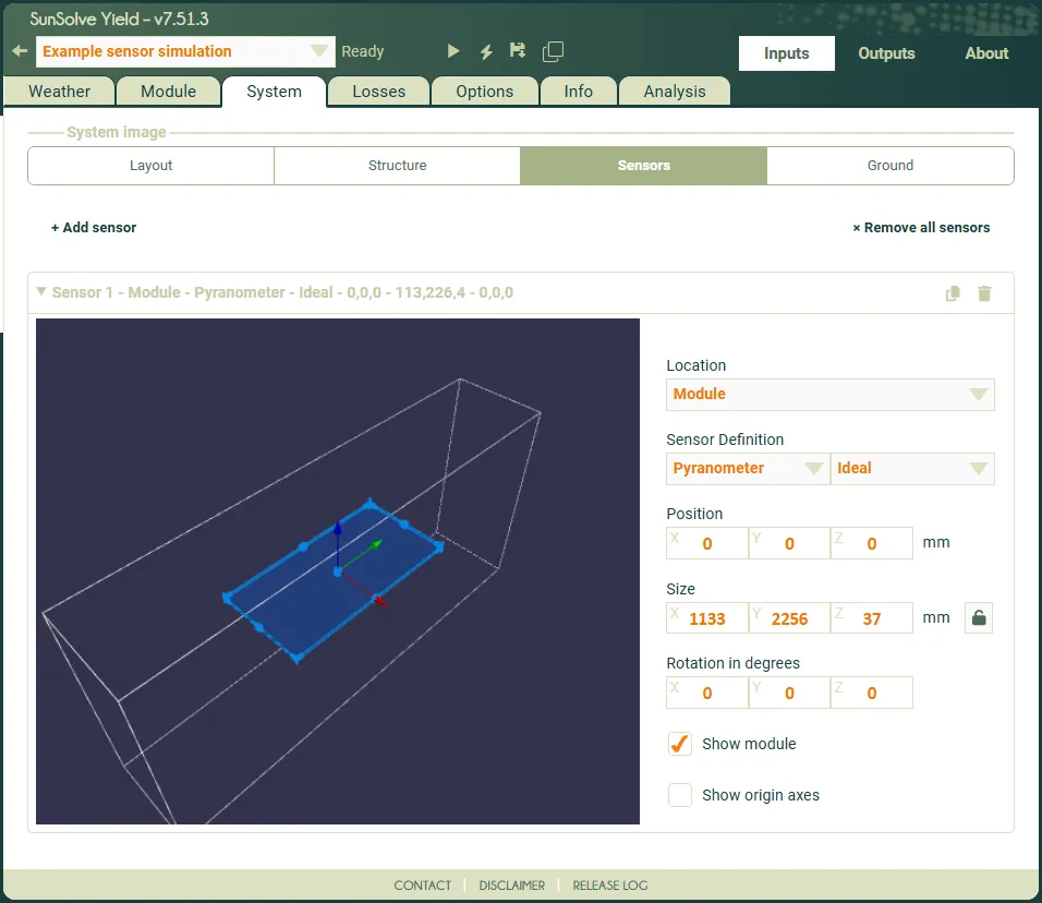
With Location set to Module, the sensor is positioned relative to the module’s geometric centre, including its frame dimensions. It also rotates about the module’s axis of rotation. Because there is more than one module in the scene, multiple sensors are created, one per module.
The sensor has two active faces: light blue on the front and red on the rear. When it overlaps the module, these faces align with the module surfaces.
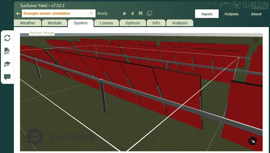
In the configuration we have used in this step it will block any light from reaching the module. Thus we expect the modules to have no electrical output power.
Read the irradiance results
Section link: Read the irradiance results- Run the simulation as you would a normal simulation.
- Go to the Outputs > Sensors tab.
On this page you can view the outputs of each sensor. It displays one sensor at a time, selected at the top of the page. The values displayed are described in more detail on the sensor outputs page.
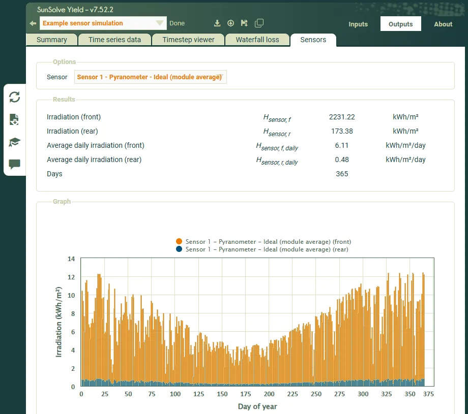
Note that for this simulation the rear irradiance for the whole year was 173 kWh/m² and the front irradiance was 2231 kWh/m². These values are the average across every module in the scene.
Step 2: measure the rear POA only
Section link: Step 2: measure the rear POA onlyCovering the whole module records both surfaces, but it also stops any light reaching the front of the module. It is more common to want the rear-side irradiance on its own, with the front of the module left exposed.
To do this, keep the sensor on the Module location and change its size and position so that it sits just behind the module.
Move the sensor behind the module
Section link: Move the sensor behind the module- Leave the Location of the sensor set to Module.
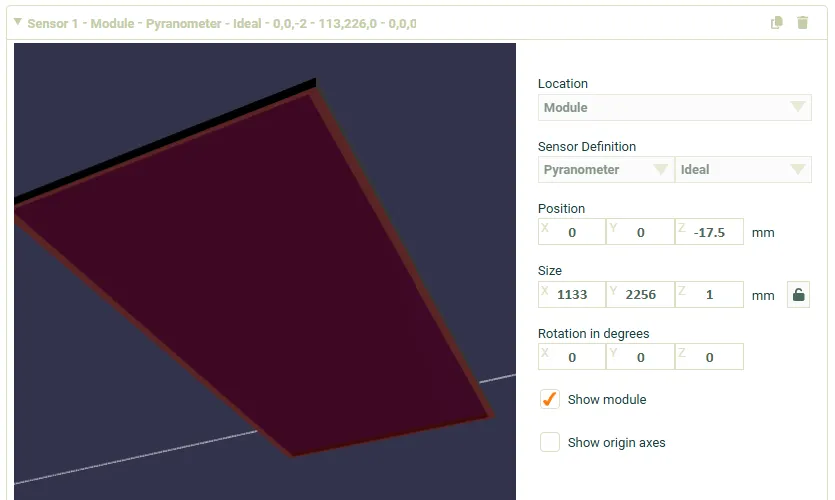
- Set the sensor Size to match the module dimensions in X and Y.
- Set the sensor Size in the Z dimension to 1 mm.
- Set Position Z = -17.5 mm. This will set the Z height of the sensor to rest against the back of the module.
The Z position value of 17.5 mm is exactly half the module thickness. Since the position is defined relative to the geometric centre of the module, this offset will place the centre of the sensor exactly at the lower edge of the module. The thickness of the module can be determined by going to the Input > Module tab and reading the dimension from the summary strip under the selected module.
Now the rear face of the sensor is between the frame of the module and the clamps and other structure beneath it. The rear face of the sensor therefore sits 0.5 mm below the frame, with the centre of the 1 mm thick sensor aligned with the rear surface of the frame. This small amount of overlap ensures the sensor is always above the frame for all angles of rotation.
Read the irradiance results
Section link: Read the irradiance resultsRun the simulation and open the Outputs > Sensors tab as before.
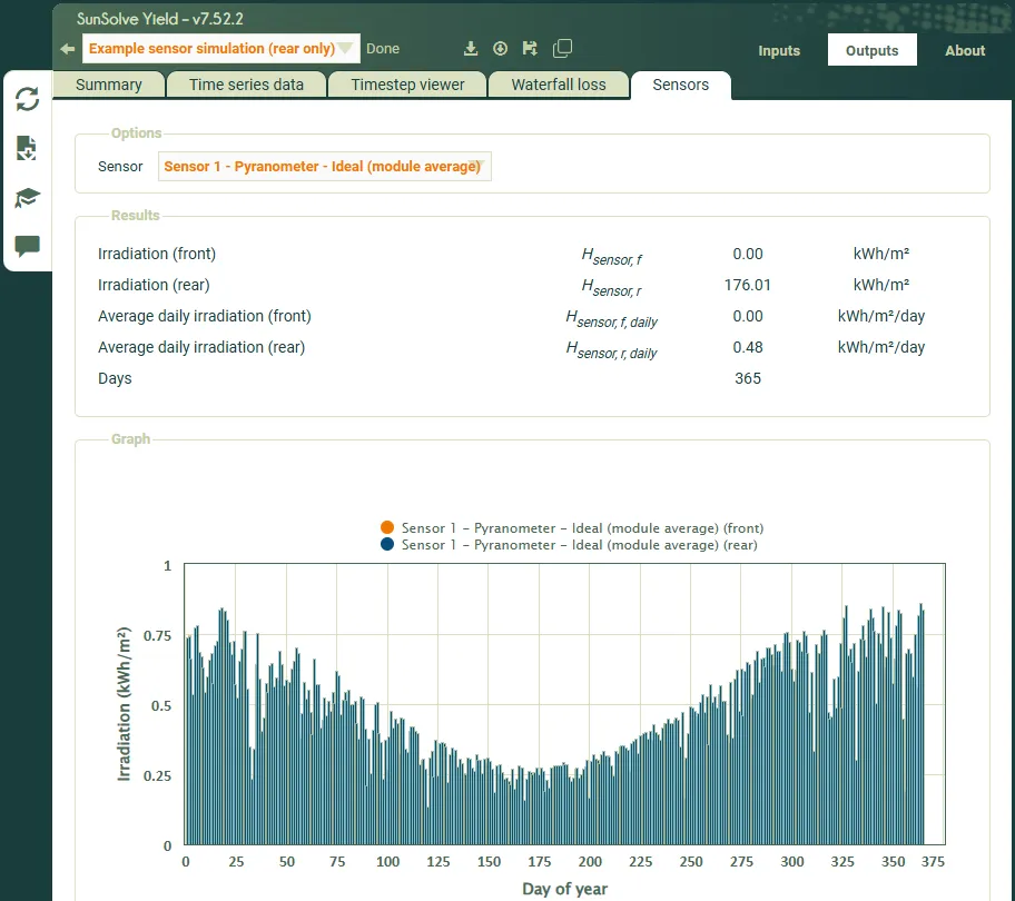
Note that for this simulation the rear irradiance for the whole year was 176 kWh/m² and the front irradiance was 0 kWh/m². The front irradiance is zero as the front face of this sensor is now positioned behind the module and therefore does not receive any light. The rear irradiance is slightly higher than in step 1. The reason is that the front side optics of the module are not covered by a sensor in this scene. Reflection from the module frames on the rows either side of the module under test has been collected by the rear-side sensor.
Step 3: measure one specific module
Section link: Step 3: measure one specific moduleSteps 1 and 2 report the average across every module in the scene. It may also be desirable to simulate the irradiance at one position in the array instead. For example to see how a module at the edge of a bay differs from one in the middle.
To do this the sensor is attached to the tracking node rather than to the module. This also demonstrates the application of sensors generally to the tracking node.
Move the sensor onto the tracking node
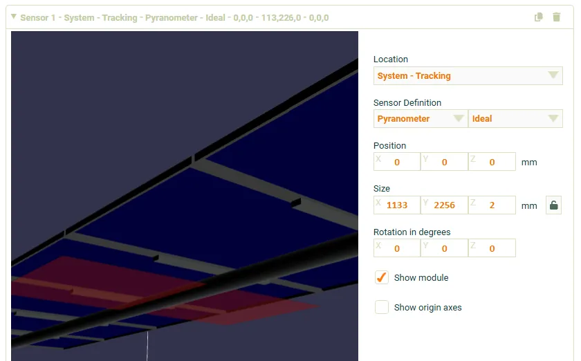
Section link: Move the sensor onto the tracking node- Change the Location of the sensor to System - Tracking.
When the sensor is added to the tracking node, or the fixed node, it is only placed once within the scene. To apply multiple sensors in this way requires new sensors to be added and positioned as needed.
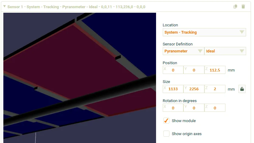
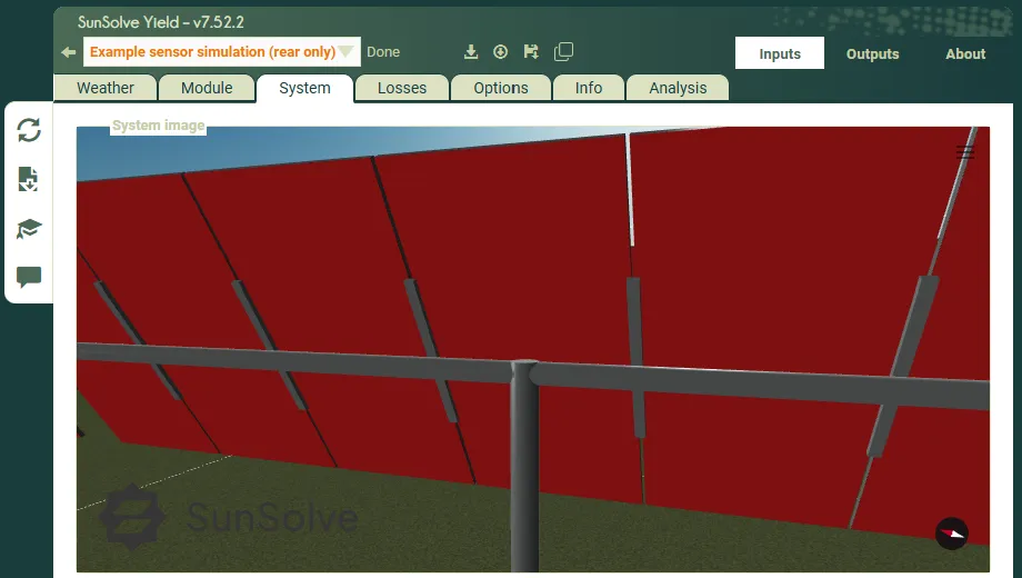
Note that at this point the sensor is centred on the axis of rotation for the tracking node. For most tracking systems that is the centre point of the torque tube. Thus in this example the sensor appears to have the torque tube cut directly through it.
Set the height of the sensor
Section link: Set the height of the sensorThe sensor is now measured from a different origin, so the Z offset used in step 2 no longer applies.
- Set Position Z = 112.5. This will set the Z height of the sensor to rest against the back of the module.
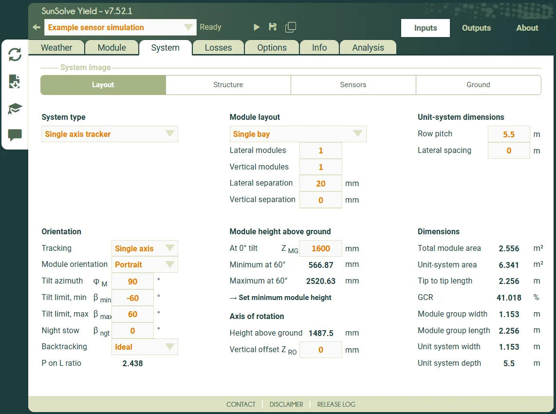
The value of Z used here to achieve this is the distance between the axis of rotation and the back of the module. That value can be determined from the Inputs > System > Layout tab. It is the difference between the height of the axis of rotation (ZRO = 1487.5 mm) and the height of the module at 0° tilt (ZMG = 1600 mm).
Choose which module to measure
Section link: Choose which module to measureThe sensor sits at the origin of the tracking node, which is the centre of the row. It will only line up with a module on its own where the scene happens to be symmetric about that point.
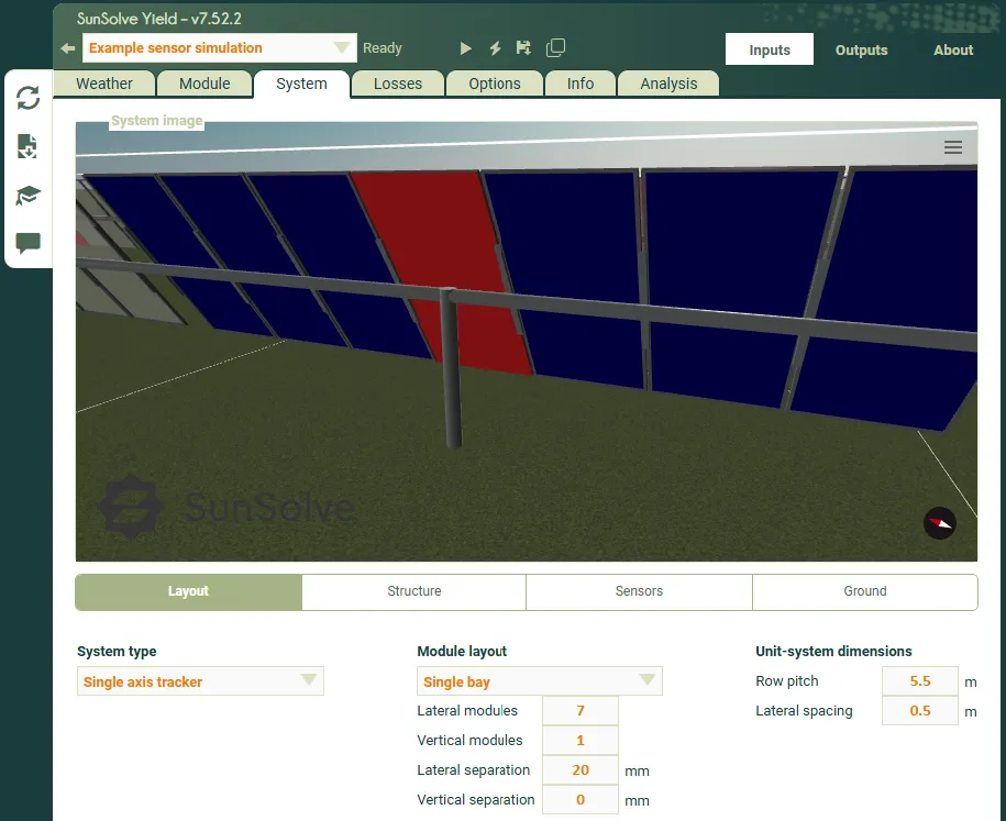
The alignment to the module in the screenshot above occurred naturally as there are an odd number of modules in a symmetric scene. Where there is an even number of modules, or a bay space in the middle region, the sensor and the module will not align properly and you must offset the sensor yourself.
As an example of how to reposition the sensor, we will move the sensor to the edge module.
- Set Position X = 3459 mm. This will reposition the sensor to align with the edge module.
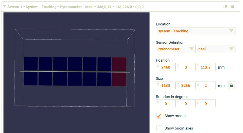
The value of X used here to achieve this was determined by considering the distance between the centre of two adjacent modules. The Inputs > Layout tab indicates a Lateral separation of the modules of 20 mm. This must be added to the module width (1133 mm) and added for each module we want to shift the sensor by. In this example we needed to make 3 such jumps and so X was set to 3 × (20 + 1133) mm = 3459 mm.
Read the irradiance results
Section link: Read the irradiance resultsRun the simulation and open the Outputs > Sensors tab as before.
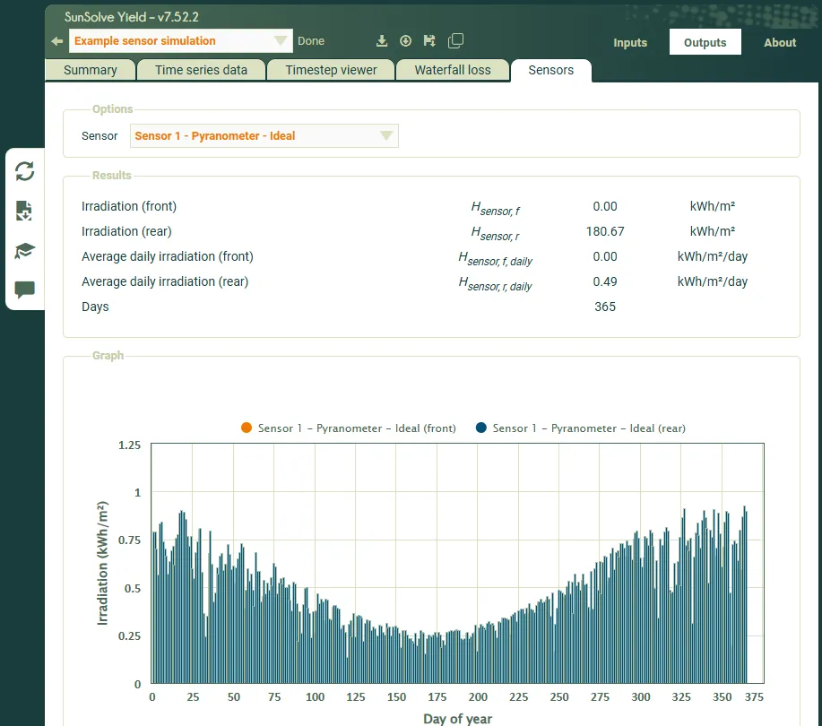
The rear irradiance for this single module was 181 kWh/m², compared with the array average of 176 kWh/m² recorded in step 2.
Comparing the results
Section link: Comparing the resultsThe values recorded in the three steps above, and the value obtained from the view factor model, are collected below. The view factor model appears once because it returns the same result in all three simulations.
Note that these results are dependent on the weather file. Your results may differ if the weather file is not the same.
Rear irradiance values are heavily dependent on the albedo. If you are comparing these results to other programs it is recommended that you convert the SunSolve system definition to use an albedo that is fixed with wavelength.
Why the three sensor results differ
Section link: Why the three sensor results differThe front irradiation is only recorded in step 1. In steps 2 and 3 the front face of the sensor sits behind the module, so it never sees the sun and reports zero.
The rear irradiation rises with each step, and each increase has a different cause.
Step 1 gives the lowest rear value because the sensor encloses the module. Its front face absorbs every ray that would otherwise have reflected off the front of the module and its frame, and some of that light would have found its way onto the rear of the modules on the neighbouring rows. Removing the front sensor in step 2 puts that reflected light back into the scene, which is why the rear value increases.
Step 3 is higher again, but for a different reason. Steps 1 and 2 report the average across all seven modules, whereas step 3 reports a single module at the end of the row. That module sits next to the lateral spacing at the edge of the bay, so more light reaches its rear than reaches a module surrounded on both sides by its neighbours. The array average is pulled down by the more enclosed modules in the middle of the row.
This is the practical lesson of the three steps. The value a sensor reports depends on what the sensor itself removes from the scene, and on where in the array it is placed. A measurement taken at one position in a real array should be compared against a sensor placed at that same position, not against the array average.
Comparing with view factor irradiance
Section link: Comparing with view factor irradianceThe sensor values can be compared to the result obtained with the simplified view-factor approach.
This value is reported for every simulation, whether or not the scene contains a sensor. It is a geometric calculation made on the module surfaces and it takes no account of the sensors, so it is identical in all three steps even though the sensors changed the light reaching the modules each time. It is therefore a fixed reference that each of the three sensor results can be measured against.
Browse to the Outputs > Waterfall tab. The top section of this chart shows the irradiance calculated with the view-factor approach.
Hover your mouse over the rear irradiance and check the value. Alternatively, scroll to the bottom to read it directly from the table.
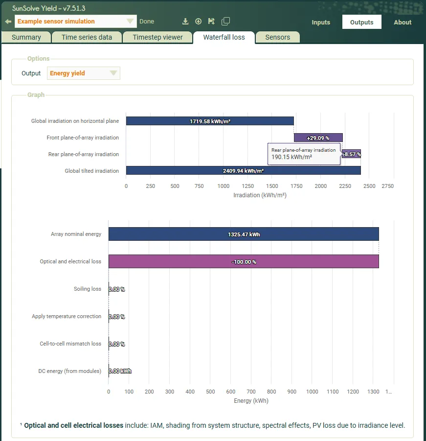
The view factor value reports an average rear irradiance for all modules of 190 kWh/m². That is around 10% above the enclosing sensor of step 1 and around 8% above the rear-only sensor of step 2, which is the closer comparison since both report the average across the whole array.
The results on the front-side are much closer. The view factor model reports 2220 kWh/m², a difference to the ray tracing result of around 0.5%.
There are a number of reasons for the difference in irradiance between view factor and ray tracing. Most significantly the view factor model does not account for the reflection and shading of the system structure. This mostly affects the rear-side, which is why the rear difference is far larger than the front. If you return to the system tab you can observe how the tracking torque tube and the clamps that attach the module to the tracker are creating shading on the sensor.
The view factor model is by its nature simplified and does not include many other detailed effects including spectral effects in the scene and the gaps between modules. The ray tracing on the other hand, when applied over a full year, solves using discrete solar arcs and a process of interpolation. This can lead to some deviation at higher incidence angles, particularly when the sun is low in the sky.
Downloading irradiance values per timestep
Section link: Downloading irradiance values per timestepThe hourly results from all sensors can be downloaded in a CSV file.
- Go to the Outputs > Time series data tab.
- Set the options as seen in the screenshot below and click Request data.
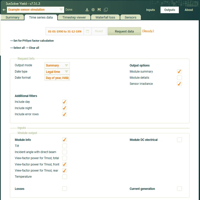
A CSV file will download with columns for both the view factor irradiance and the sensor irradiance values.
Summary: choosing a configuration
Section link: Summary: choosing a configurationEvery configuration in this guide comes down to two independent choices.
- Where the sensor is attached. This sets which modules you measure. Attaching the sensor to the module places one on every module in the scene. Attaching it to the tracking node, or the fixed node, gives a single sensor that you position against a specific module.
- How the sensor is sized and positioned. This sets which surfaces you measure. Sizing the sensor so that it encloses the module records the front and rear irradiance at the same time. Leaving the sensor thin and positioning it just behind the module records the rear irradiance only.
The two choices are made independently, so any combination of them is valid.
Rear POA only on one chosen module, System - Tracking or System - Fixed, Thin sensor just behind the module
The three steps above walk through the first, the second and the fourth of these combinations. The third is built the same way, by combining the sizing from step 1 with the location and offsets from step 3.